Building a Movie Recommendation App with ScyllaDB Vector Search
Use ScyllaDB to perform semantic search across movie plot descriptions We built a sample movie recommendation app to showcase ScyllaDB’s new vector search capabilities. The sample app gives you a simple way to experience building low-latency semantic search and vector-based applications with ScyllaDB. Join the Vector Search Early Access Program In this post, we’ll show how to perform semantic search across movie plot descriptions to find movies by meaning, not keywords. This example also shows how you can add ScyllaDB Vector Search to your existing applications. Before diving into the application, let’s clarify what we mean by semantic search and provide some context about similarity functions. About vector similarity functions Similarity between two vectors can be calculated in several ways. The most common methods are cosine similarity, dot product (inner product), and L2 (Euclidean) distance. ScyllaDB Vector Search supports all of these functions. For text embeddings, cosine similarity is the most often used similarity function. That’s because, when working with text, we mostly focus on the direction of the vector, rather than its magnitude. Cosine similarity considers only the angle between the vectors (i.e., the difference in directions) and ignores the magnitude (length of the vector). For example, a short document (1 page) and a longer document (10 pages) on the same topic will still point in similar directions in the vector space even though they are different lengths. This is what makes cosine similarity ideal for capturing topical similarity. Cosine similarity formula In practice, many embedding models (e.g., OpenAI models) produce normalized vectors. Normalized vectors all have the same length (magnitude of 1). For normalized vectors, cosine similarity and the dot product return the same result. This is because cosine similarity divides the dot product by the magnitudes of the vectors, which are all 1 when vectors are normalized. The L2 function produces different distance values compared to the dot product or cosine similarity, but the ordering of the embeddings remains the same (assuming normalized vectors). Now that you have a better understanding of semantic similarity functions, let’s explain how the recommendation app works. App overview The application allows users to input what kind of movie they want to watch. For example, if you type “American football,” the app compares your input to the plots of movies stored in the database. The first result is the best match, followed by other similar recommendations. This comparison uses ScyllaDB Vector Search. You can find the source code on GitHub, along with setup instructions and a step-by-step tutorial in the documentation. For the dataset, we are reusing a TMDB dataset available on Kaggle. Project requirements To run the application, you need a ScyllaDB Cloud account and a vector search enabled cluster. Right now, you need to use the API to create a vector search enabled cluster. Follow the instructions here to get started! The application depends on a few Python packages: ScyllaDB Python driver – for connecting and querying ScyllaDB. Sentence Transformers – to generate embeddings locally without requiring OpenAI or other paid APIs. Streamlit – for the UI. Pydantic – to make working with query results easier. By default, the app uses the all-MiniLM-L6-v2 model so anyone can run it locally without heavy compute requirements. Other than ScyllaDB Cloud, no commercial or paid services are needed to run the example. Configuration and database connection Aconfig.py file stores ScyllaDB
Cloud credentials, including the host address and connection
details. A separate ScyllaDB
helper module handles the following: Creating the connection
and session Inserting and querying data Providing helper functions
for clean database interactions Database schema The schema is
defined in a schema.cql file, executed when running
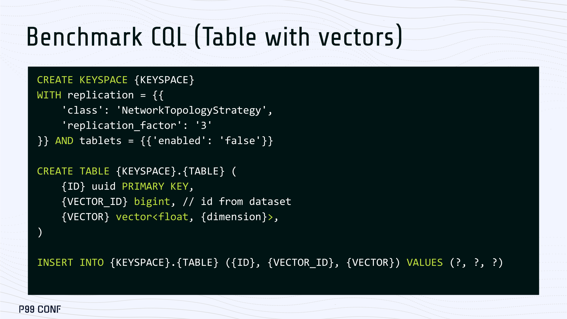
the project’s migration script. It includes: Keyspace creation
(with a replication factor of 3) Table definition for movies,
storing fields like release_date, title,
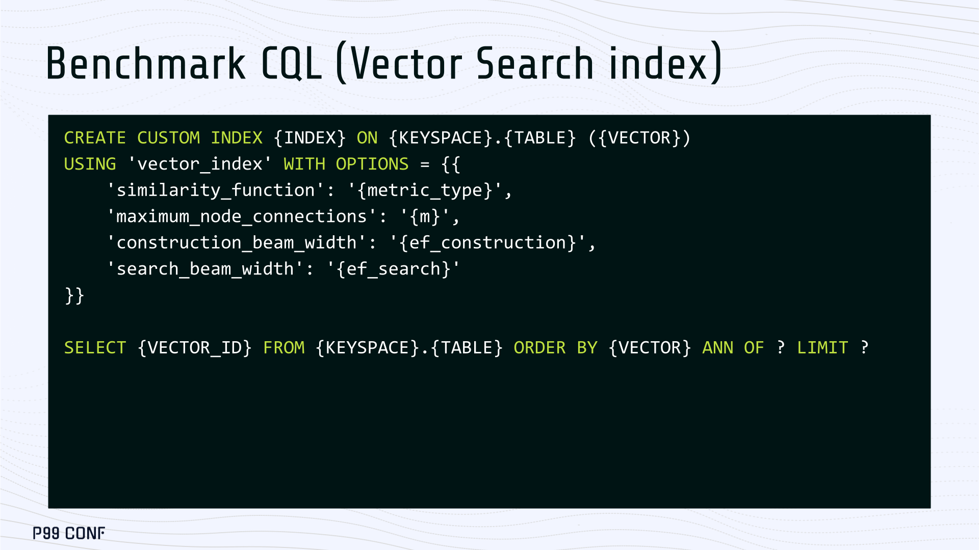
genre, and plot Vector search index
Schema highlights: `plot` – text, stores the movie description used
for similarity comparison. `plot_embedding` – vector, embedding
representation of the plot, defined using the vector data type with
384 dimensions (matching the Sentence Transformers model). `Primary
key` – id as the partition key for efficient lookups querying by id
CDC enabled – required for ScyllaDB vector search. `Vector
index` – an Approximate Nearest Neighbor (ANN) index created on the
plot_embedding column to enable efficient vector queries. The goal
of this schema is to allow efficient search on the plot embeddings
and store additional information alongside the vectors. Embeddings
An Embedding Creator class handles text embedding generation with
Sentence Transformers. The function accepts any text input and
returns a list of float values that you can insert into ScyllaDB’s
`vector` column. Recommendations implemented with vector search The
app’s main function is to provide movie recommendations. These
recommendations are implemented using vector search. So we create a
module called recommender that handles Taking the
input text Turning the text into embeddings Running vector search
Let’s break down the vector search query: SELECT * FROM
recommend.movies ORDER BY plot_embedding ANN OF [0.1, 0.2, 0.3, …]
LIMIT 5; User input is first converted to an embedding,
ensuring that we’re comparing embedding to embedding. The rows in
the table are ordered by similarity using the ANN operator
(ANN OF). Results are limited to five similar movies.
The SELECT statement retrieves all columns from the
table. In similarity search, we calculate the distance between two
vectors. The closer the vectors in vector space, the more similar
their underlying content. Or, in other words, a smaller distance
suggests higher similarity. Therefore, an ORDER BY sort results in
ascending order, with smaller distances appearing first. Streamlit
UI The UI, defined in app.py, ties everything
together. It takes the user’s query, converts it to an embedding,
and executes a vector search. The UI displays the best match and a
list of other similar movie recommendations. Try it yourself! If
you want to get started building with ScyllaDB Vector Search, you
have several options: Explore the
source code on GitHub Use the
README to set up the app on your computer Follow the
tutorial to build the app from scratch And if you have
questions, use the forum
and we’ll be happy to help. Building a Low-Latency Vector Search Engine for ScyllaDB
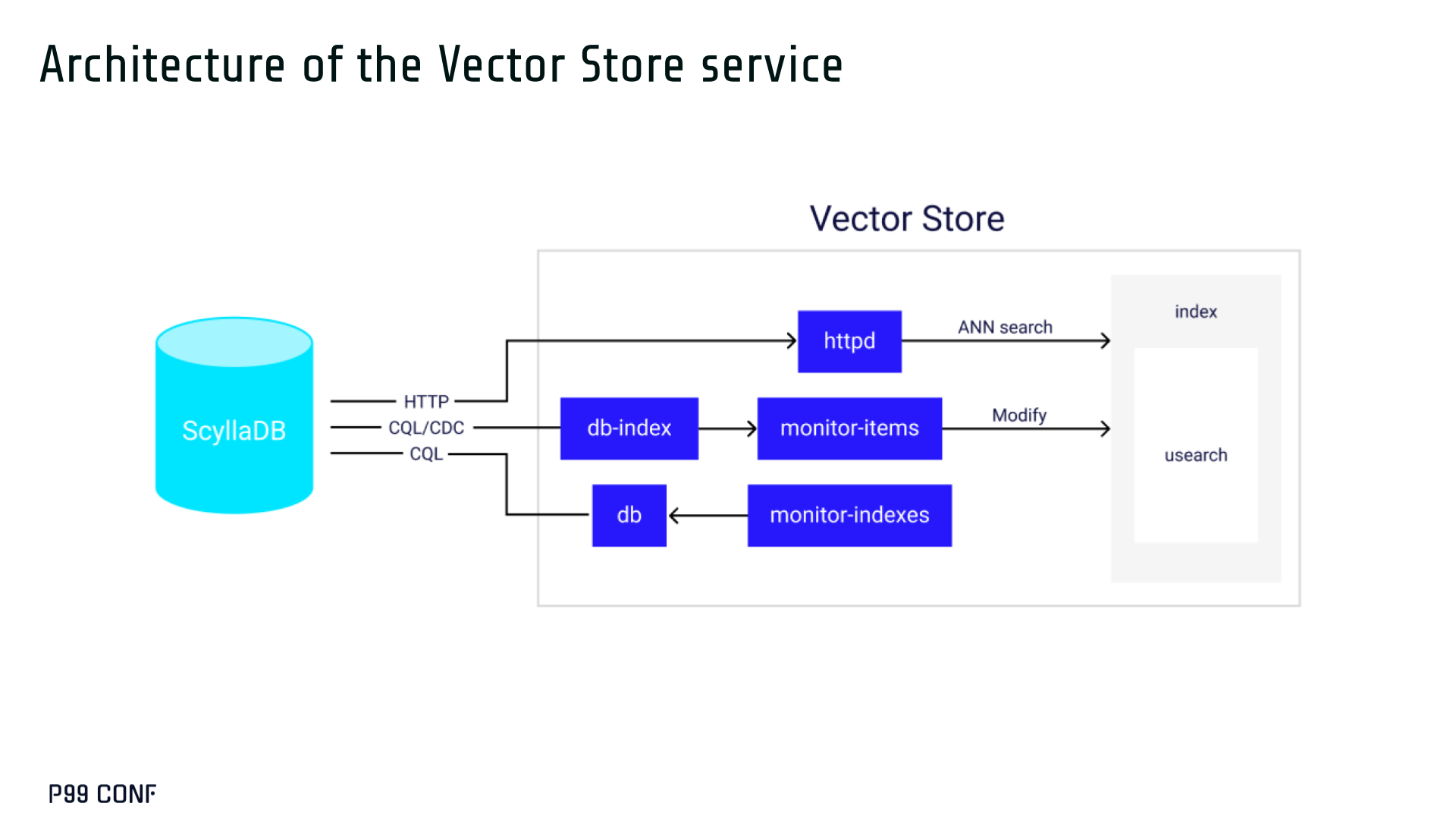
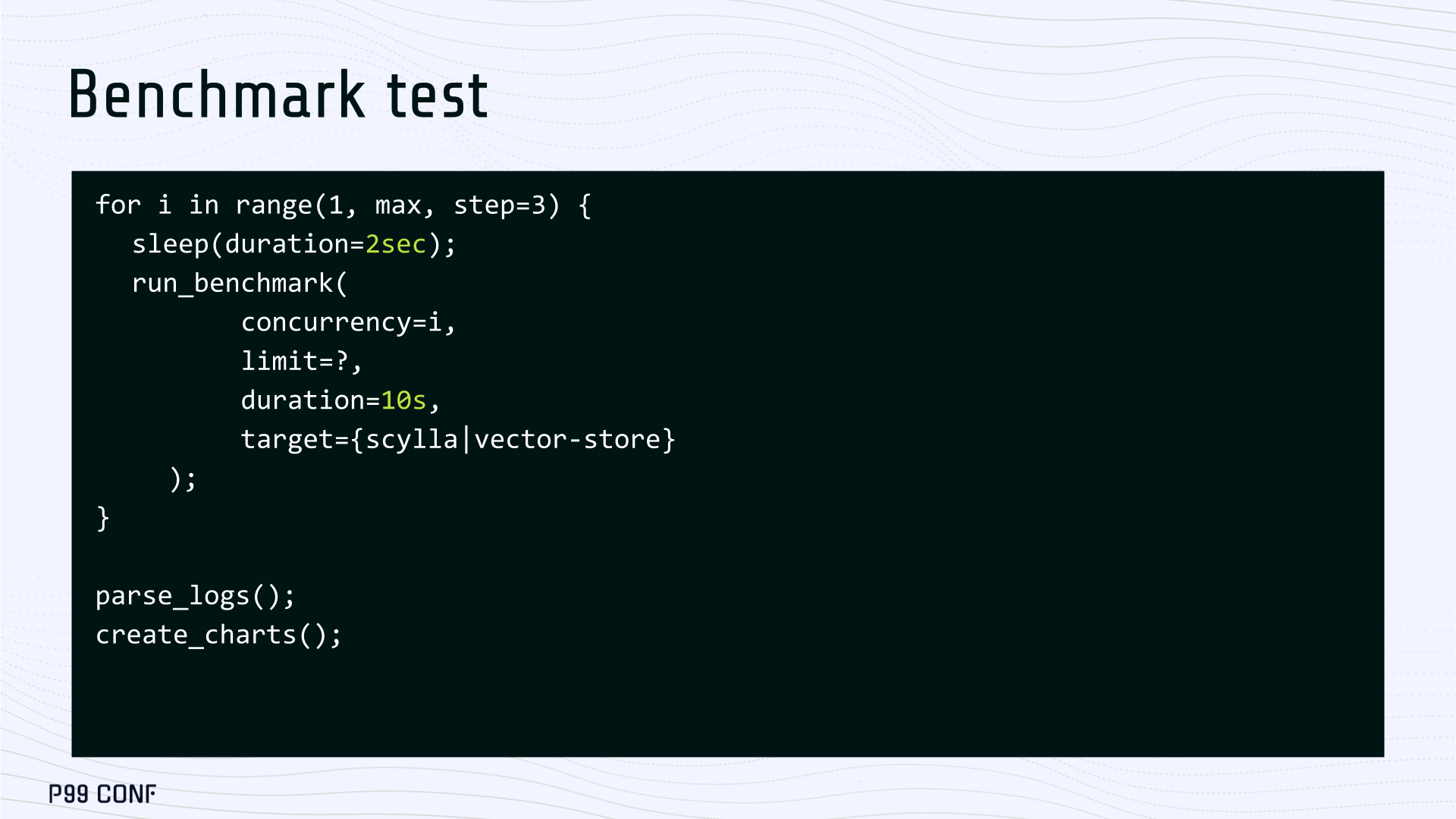
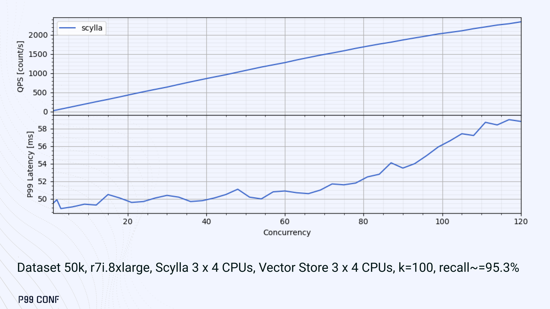
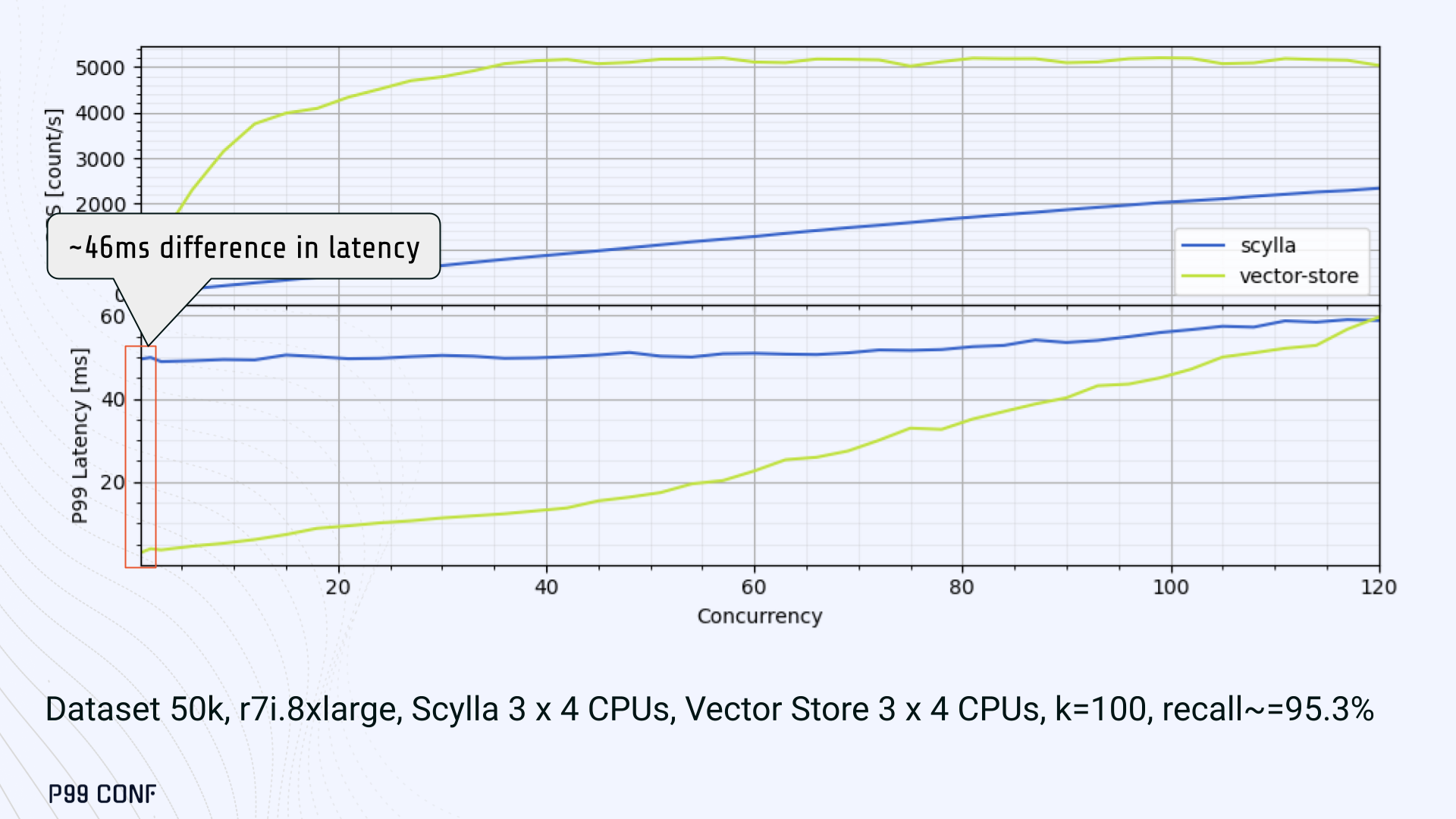
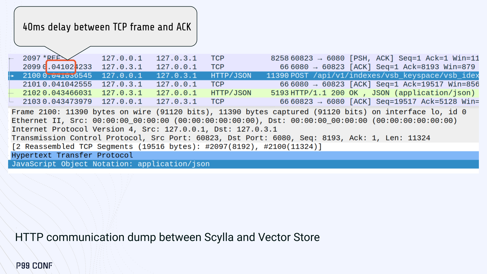
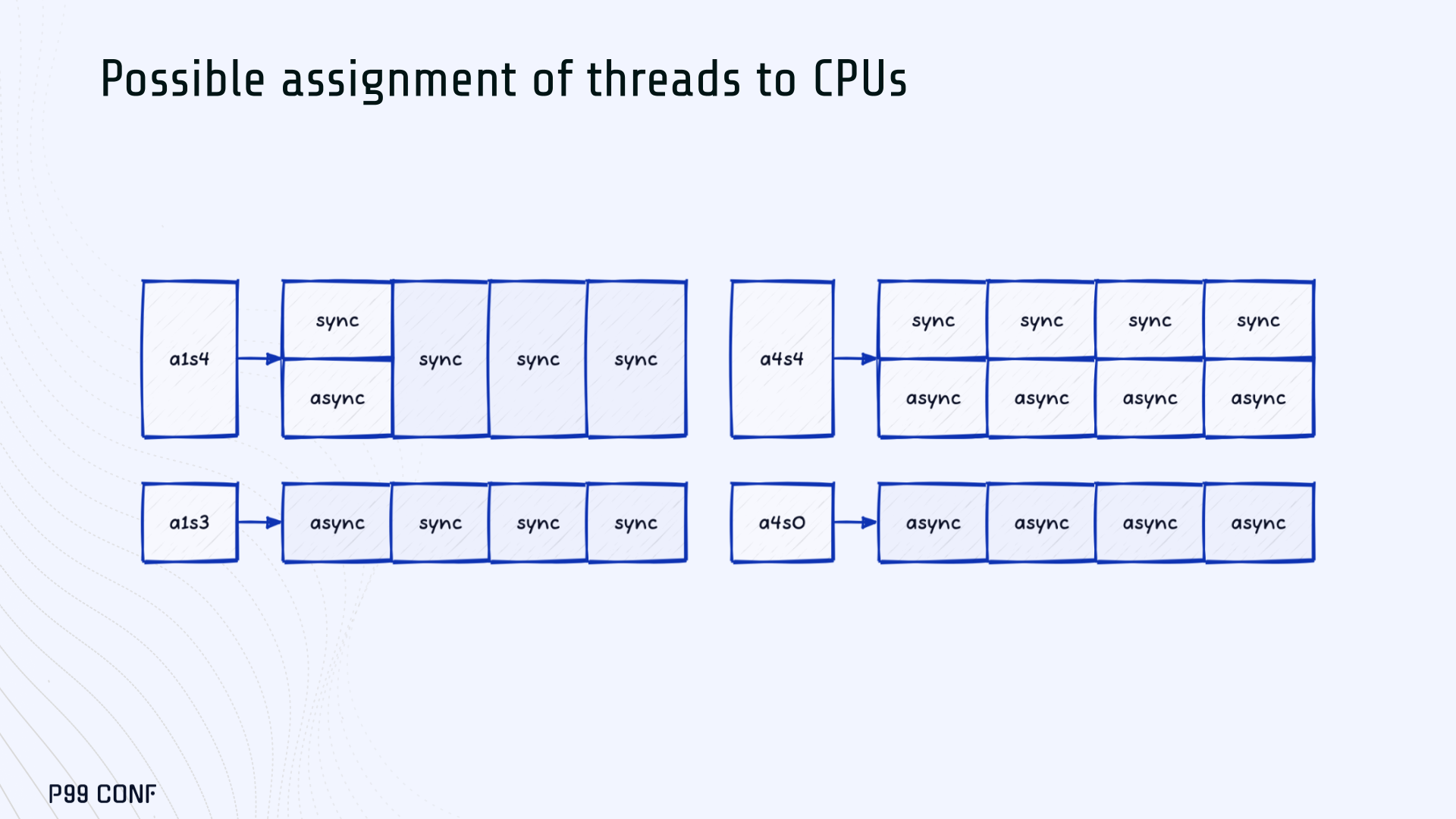
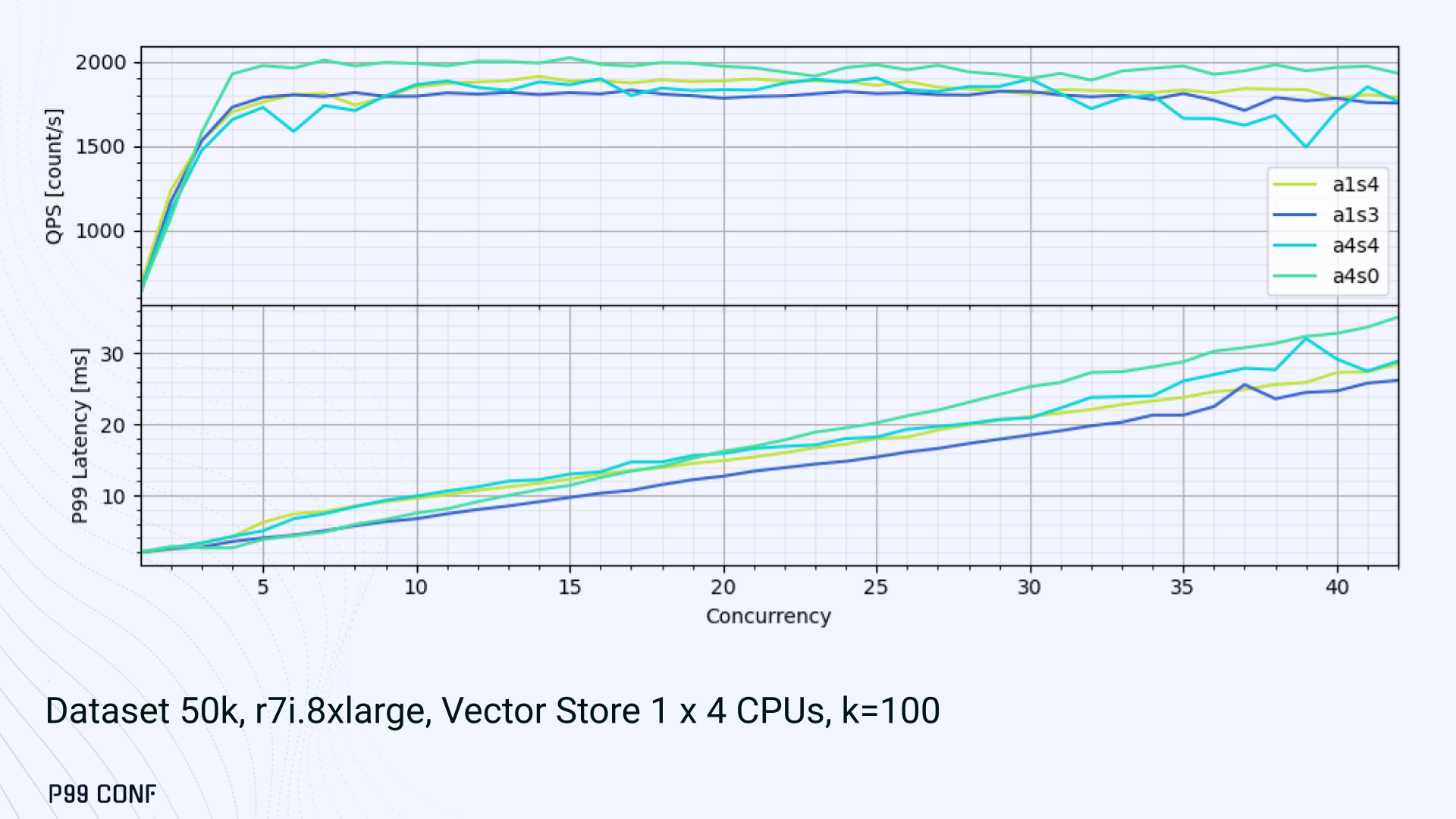
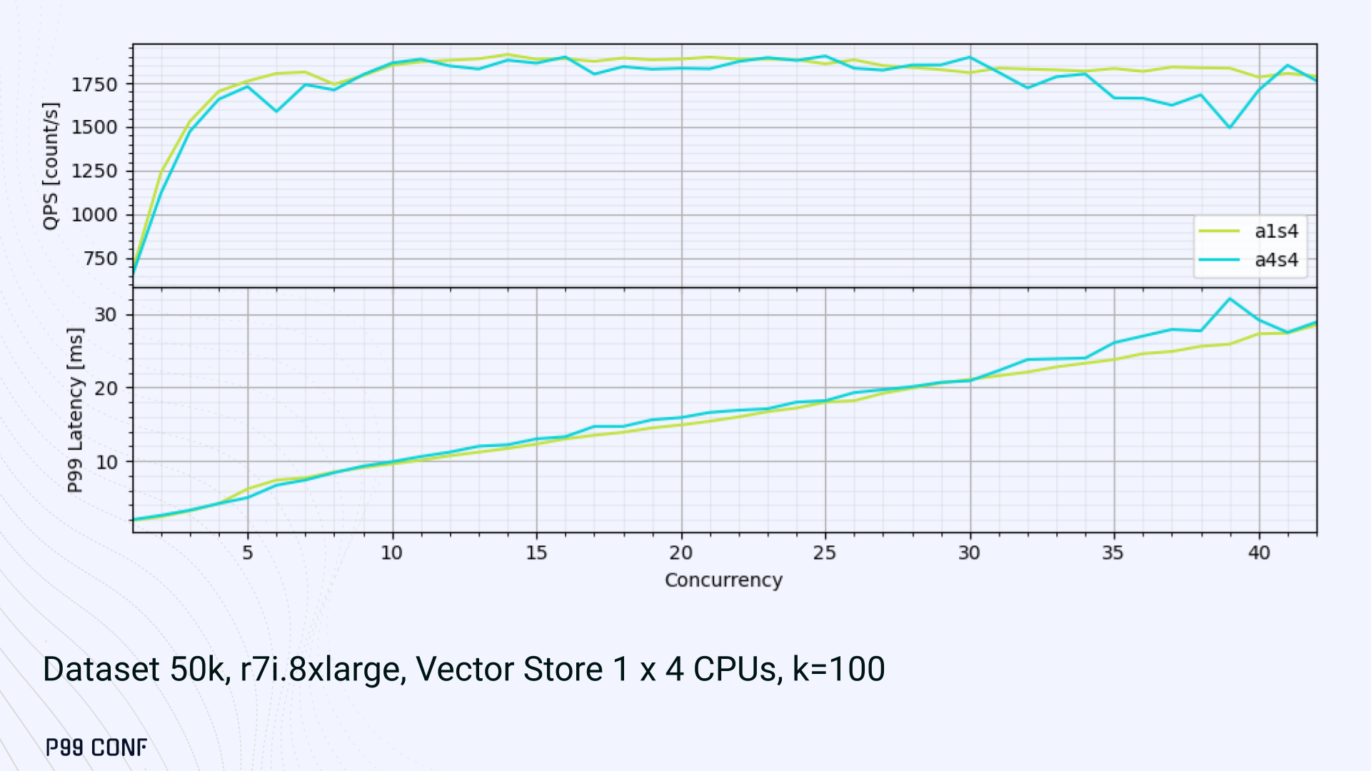
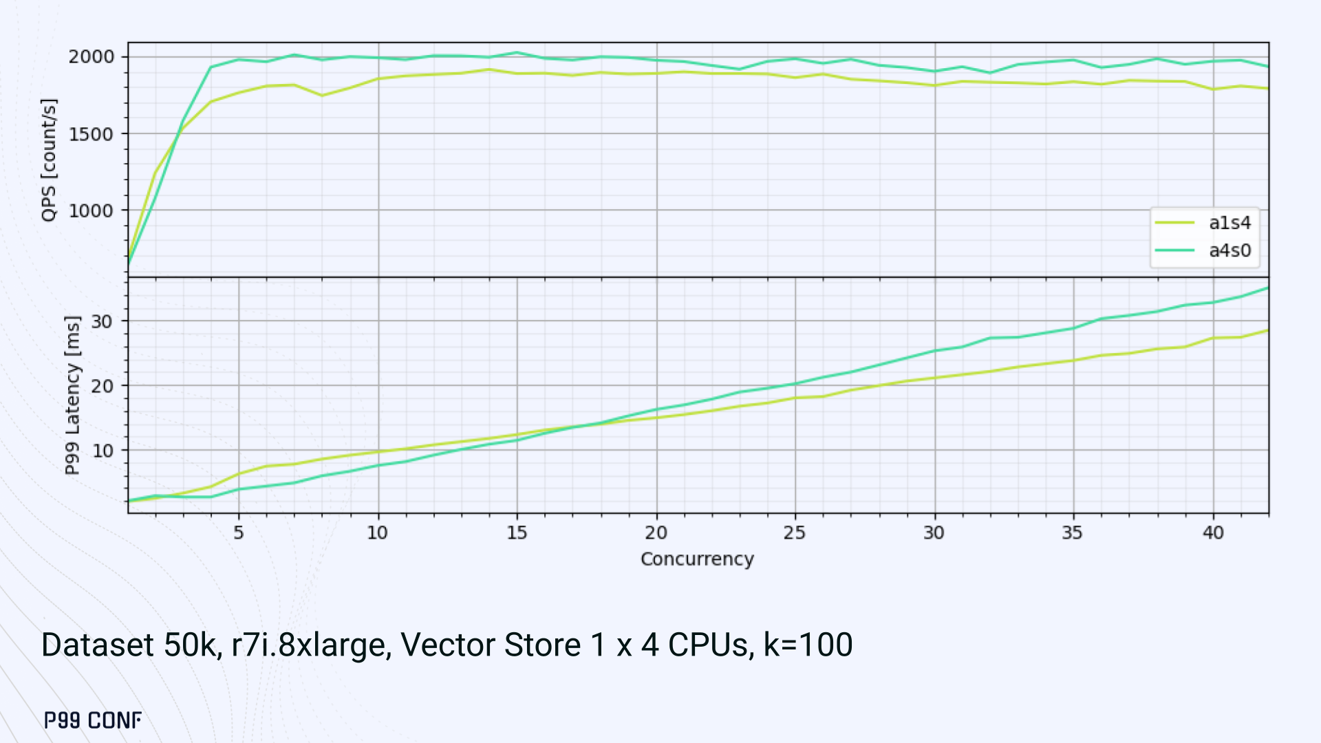
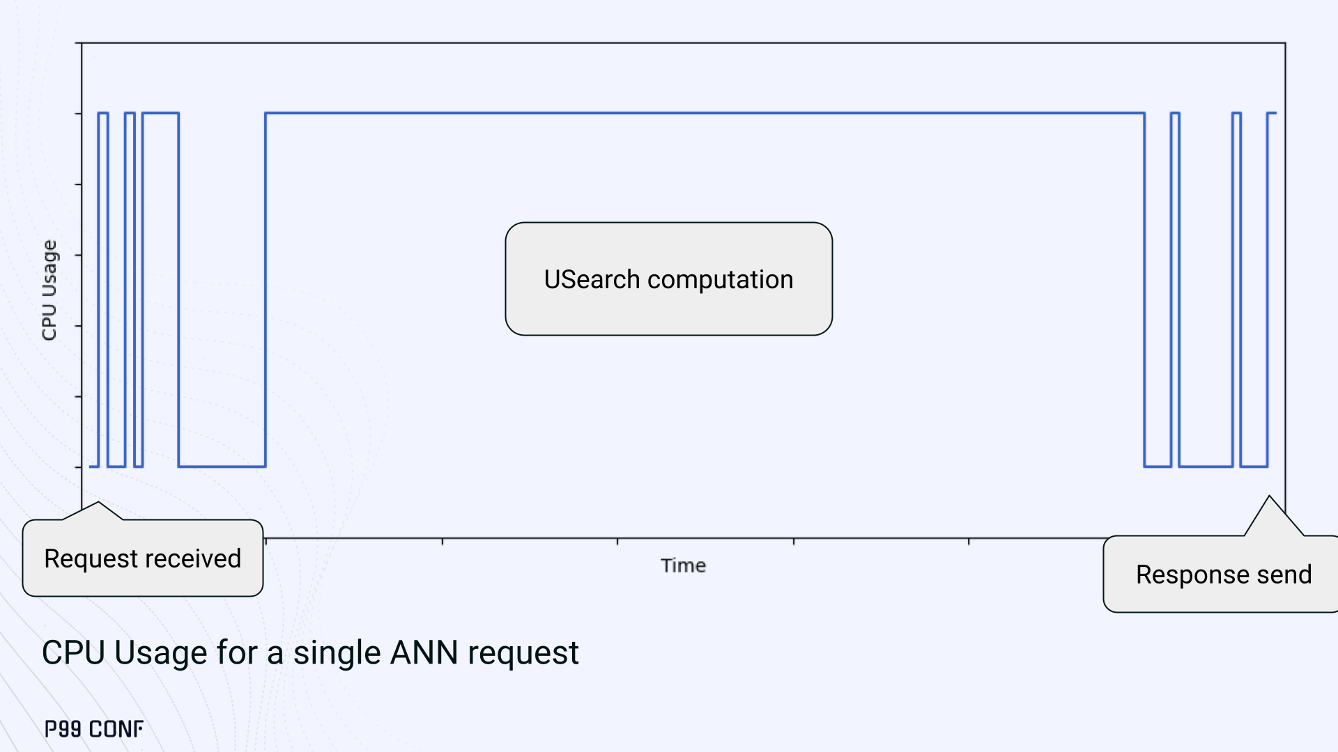
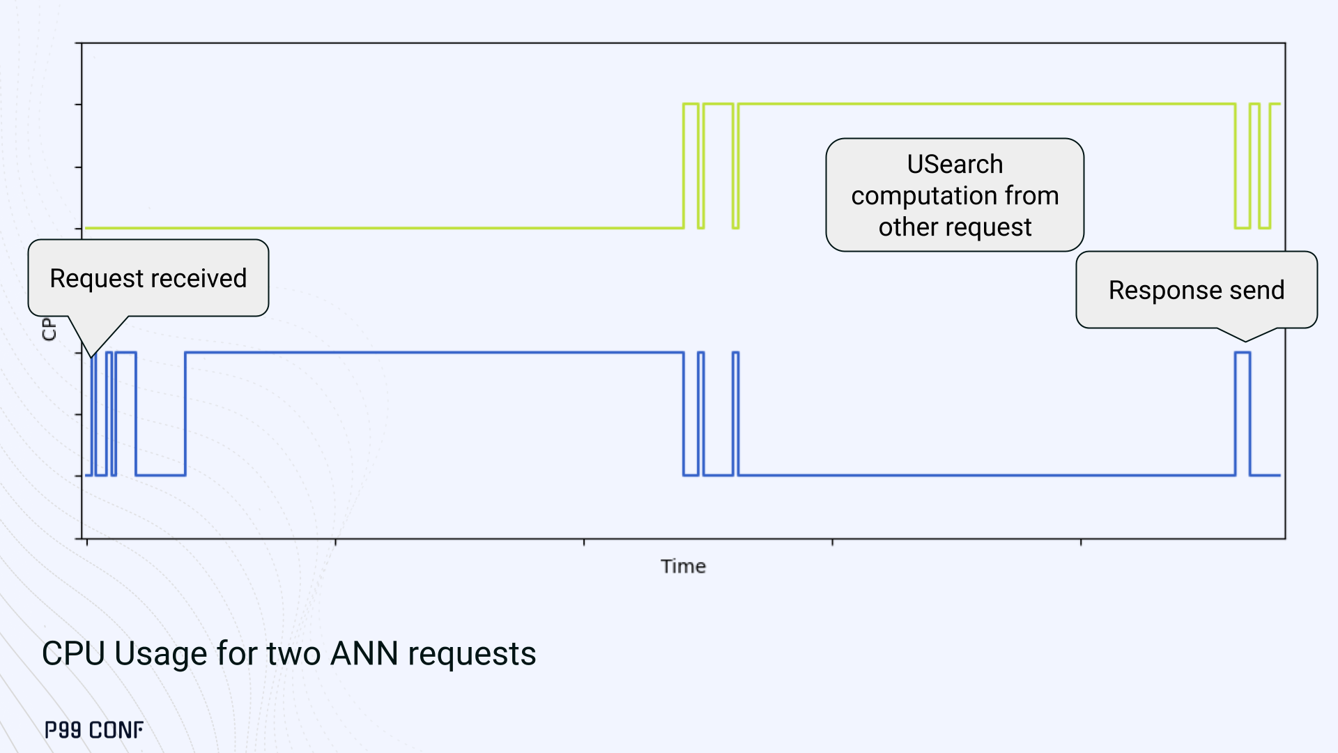
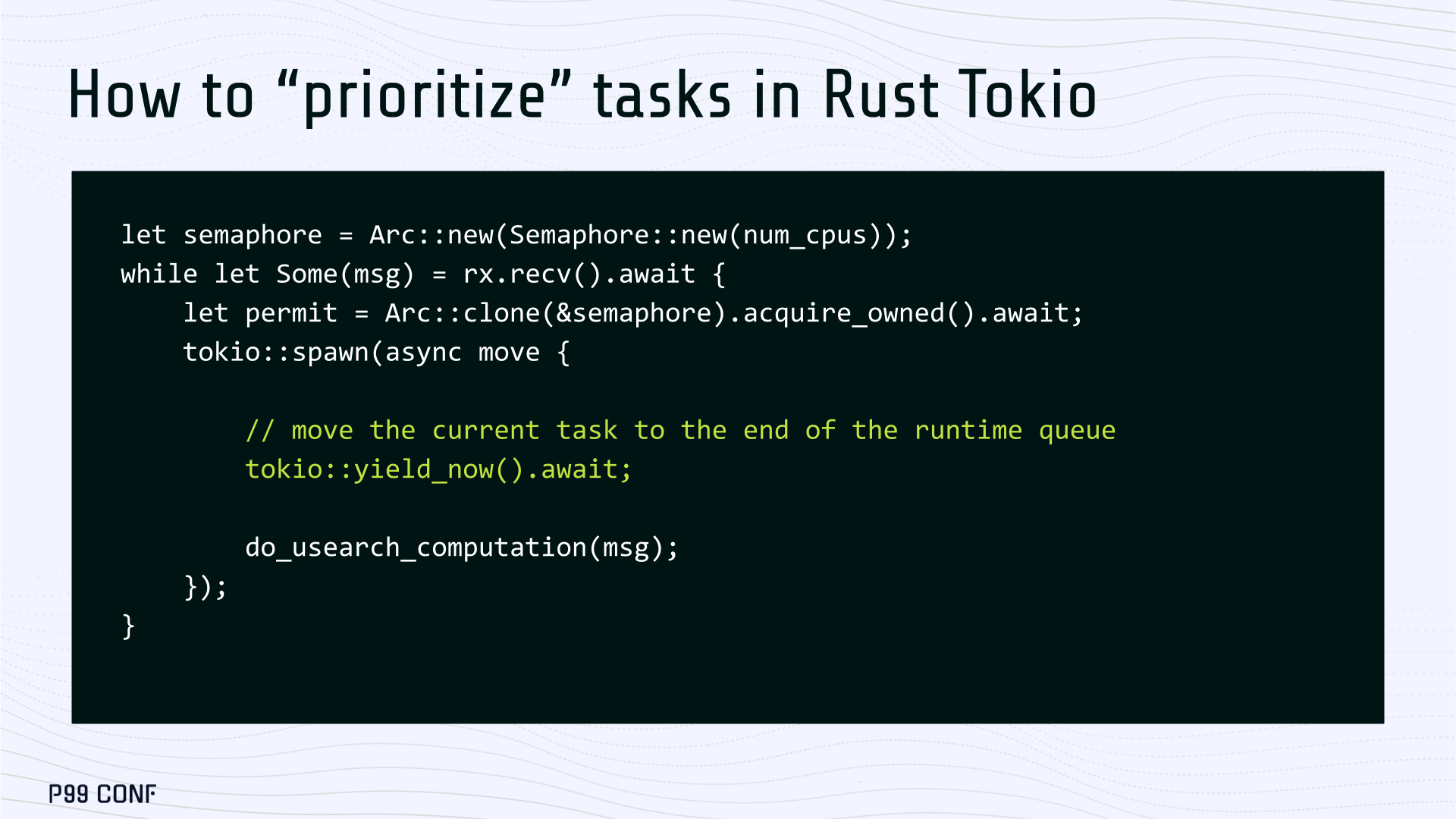
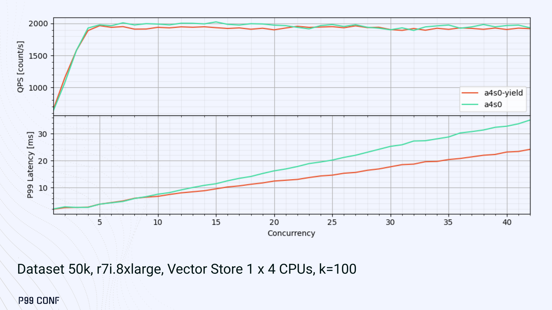
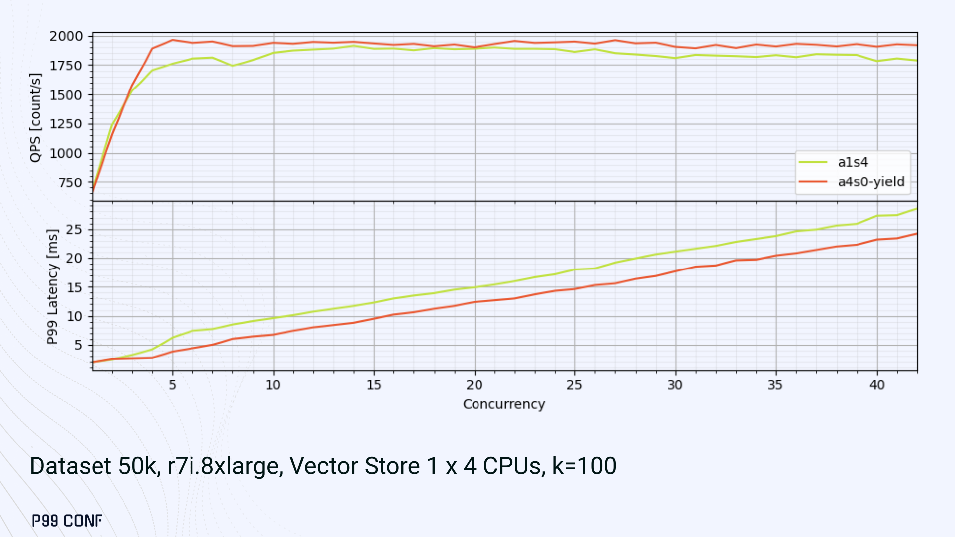
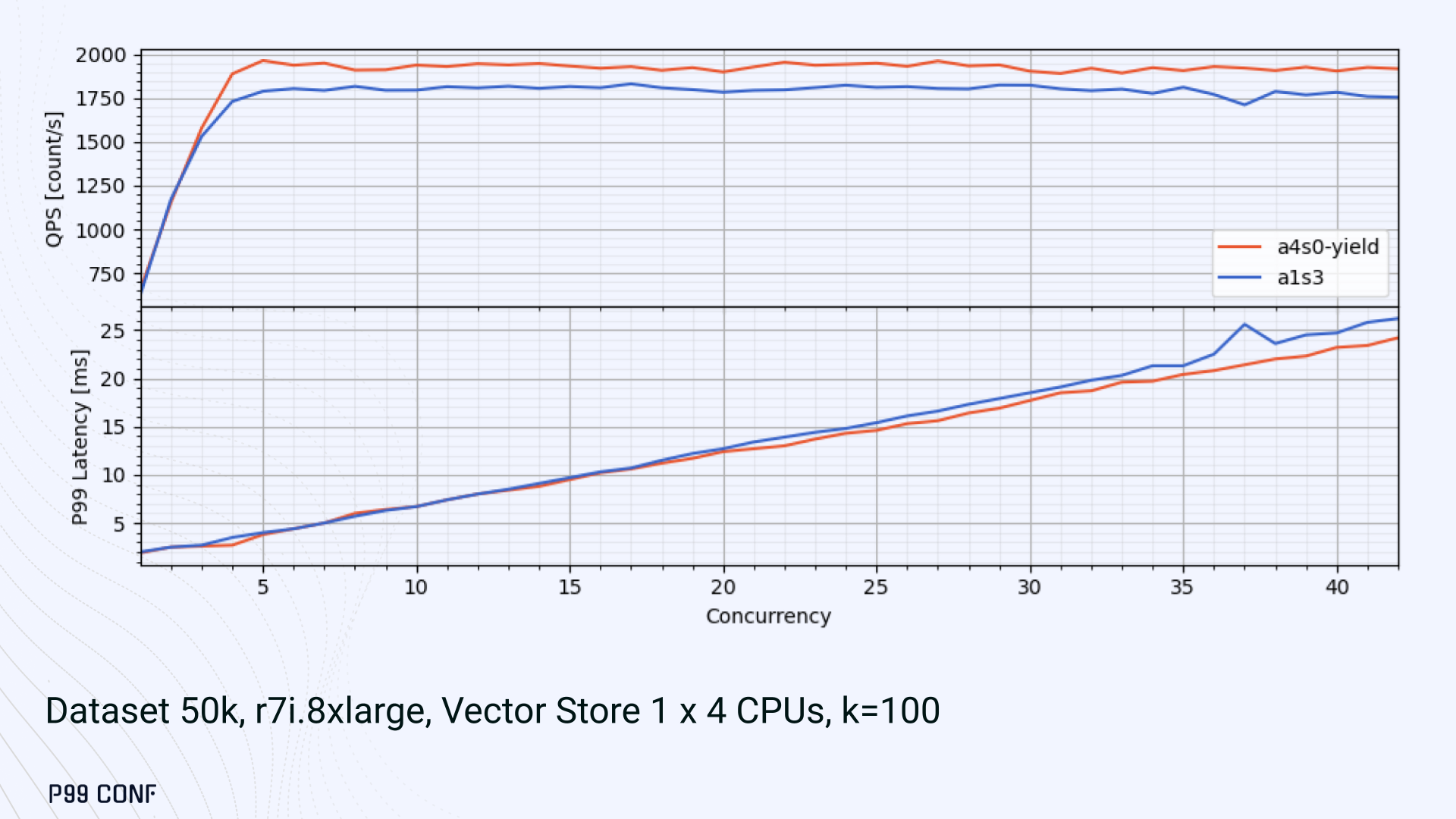
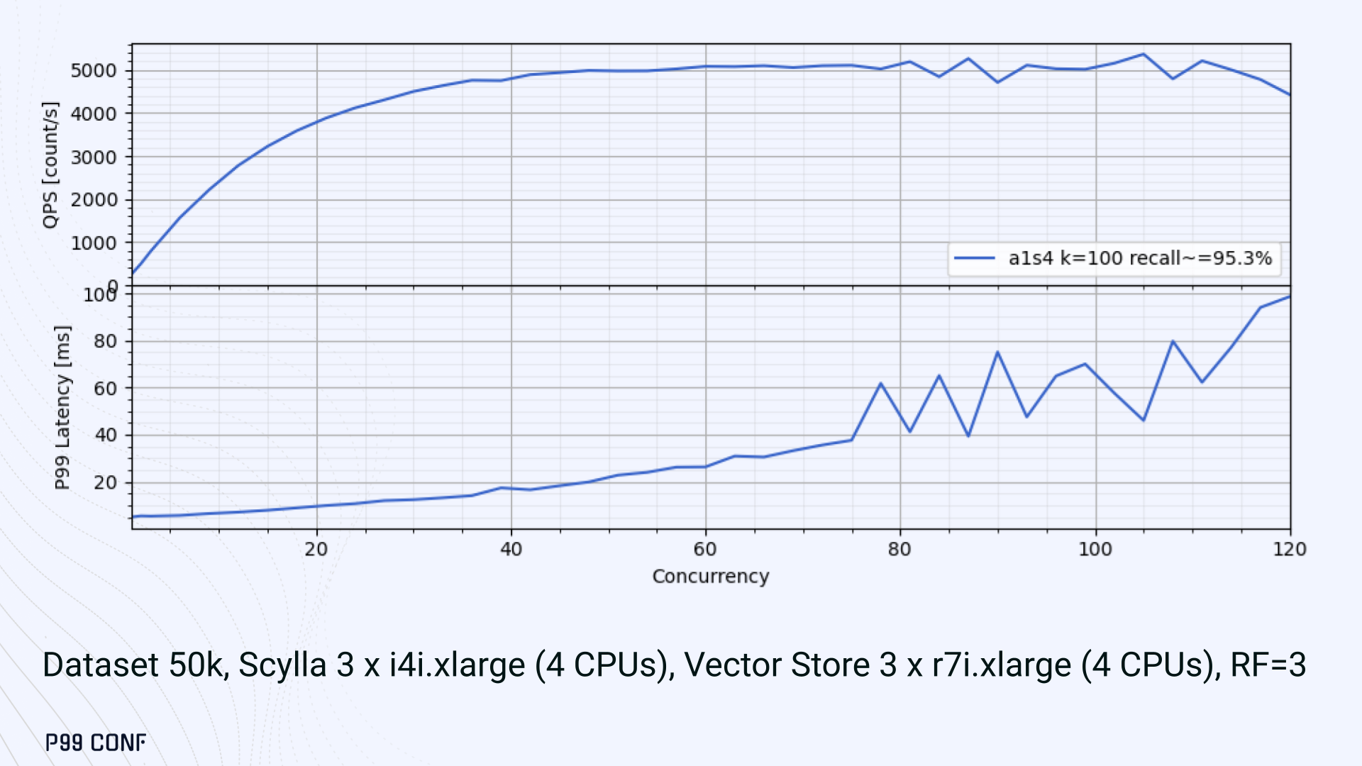
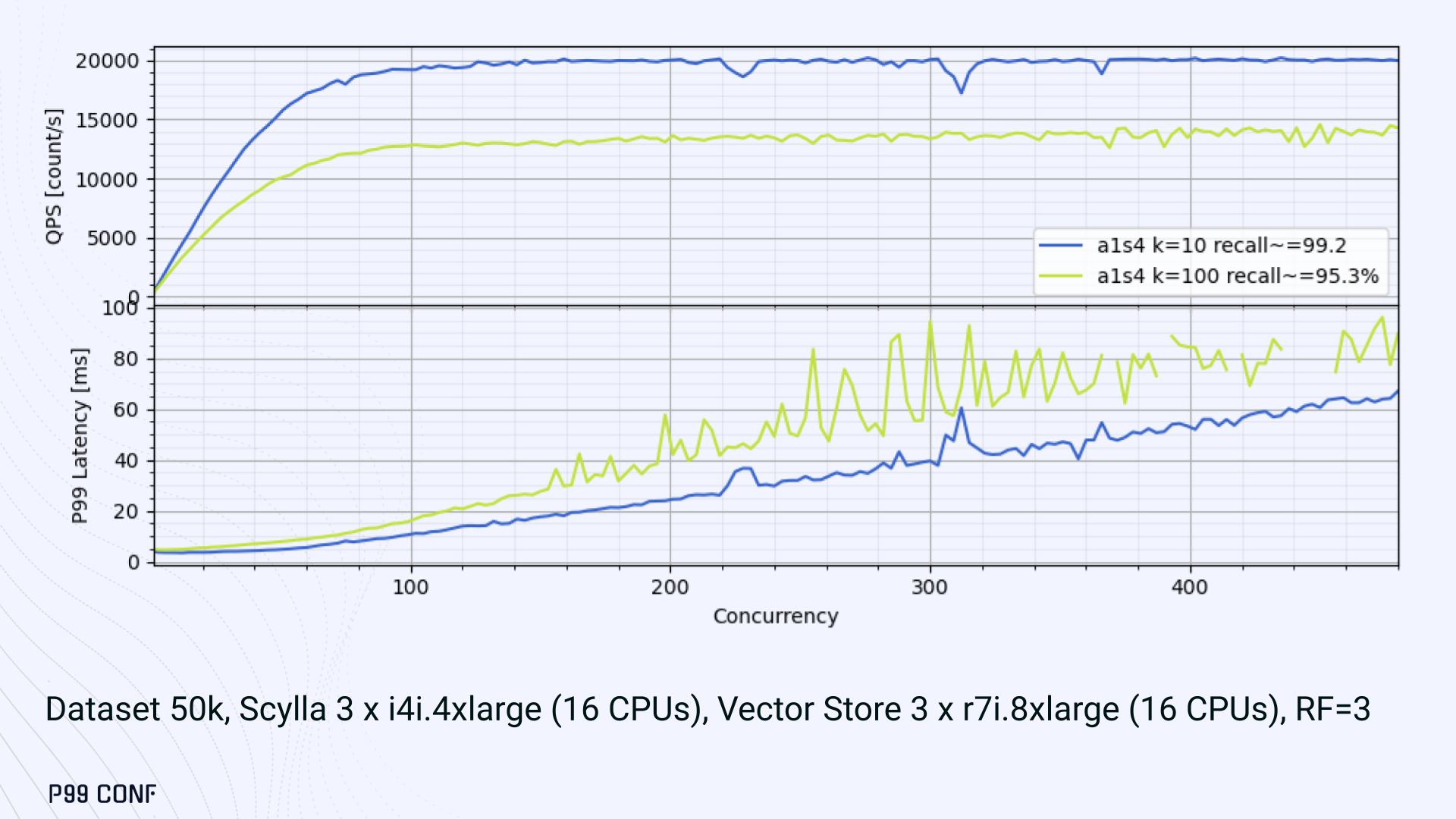
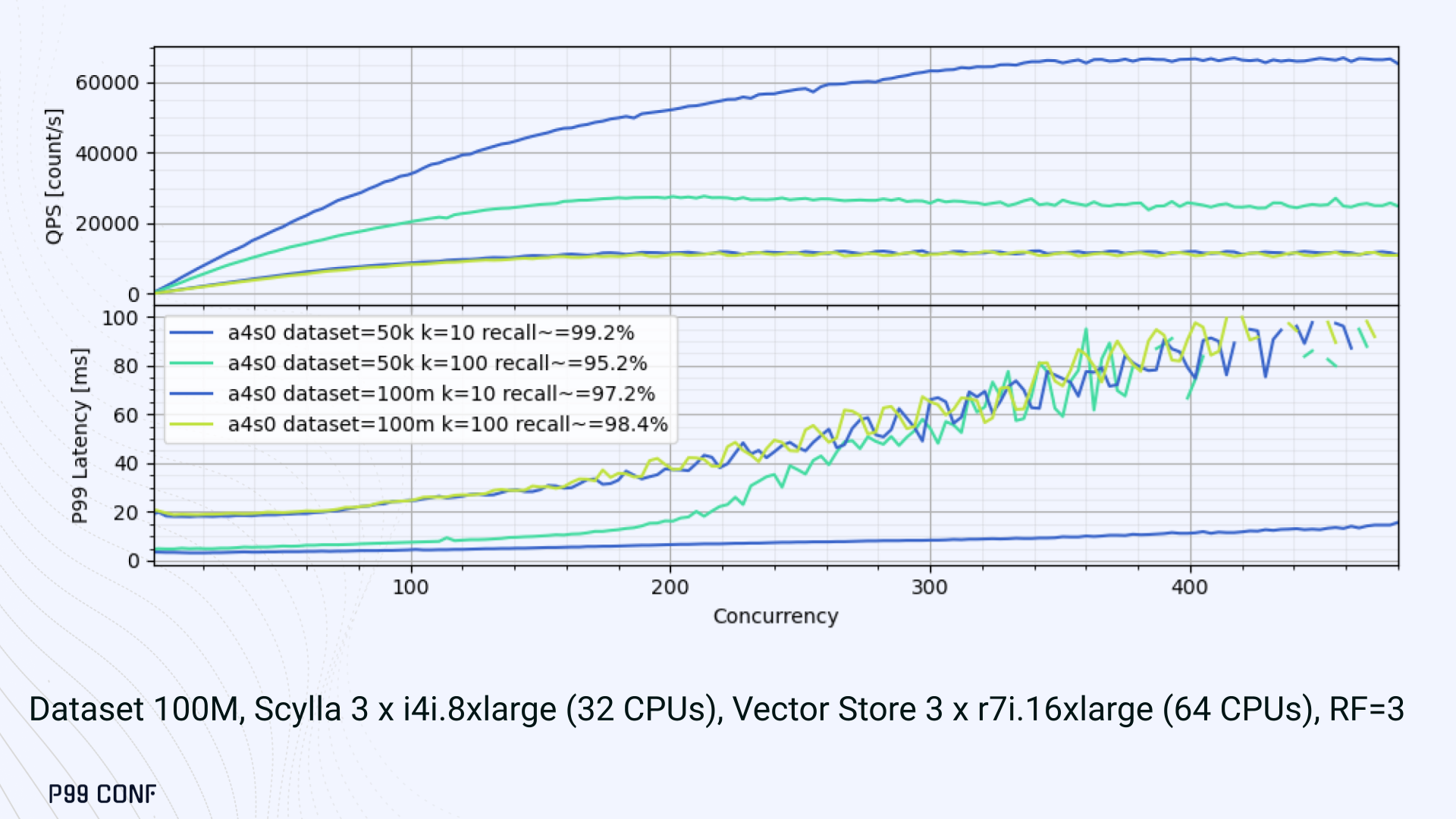
ScyllaDB Vector Search is now available. Learn about the design decisions, testing, and optimizations involved in achieving our performance goals. ScyllaDB Vector Search Beta is now available for early access. ScyllaDB Vector Search brings millisecond-latency vector retrieval to massive scale. This makes ScyllaDB optimal for large-scale semantic search and retrieval-augmented generation workloads. If you want to participate in our Early Access Program, let us know. We’d be happy to give you a product tour and answer all your questions. Join our early access program Learn more about ScyllaDB for AI In this blog post, we share a bit about what was involved in introducing low latency and high throughput Vector Search to ScyllaDB. We’ll cover the architectural design decisions behind our integration of ScyllaDB’s shard-per-core for real-time operations and high-performance ANN processing. Additionally, we’ll look at some unexpected performance challenges we encountered and how we addressed them. If you’re really just looking for some early performance numbers, here you go: ScyllaDB Vector Search outperforms industry averages in both throughput and latency. Using public VectorDBBench datasets, it sustained up to 65K QPS (P99 < 20ms) on openai_small_50k, and 12K QPS (P99 < 40ms) on laion_large_100m. Across both configurations, tests demonstrate consistently high recall accuracy and predictable latencies, even under extreme concurrency. Why Vector Search for ScyllaDB? You might be wondering why we built Vector Search for ScyllaDB. Many vendors offer Vector Search, but we had some unique goals when we started our journey. ScyllaDB’s architecture is recognized for its performance. Users have been relying on us for real-time ML, predictive analytics, fraud detection and other latency-sensitive AI workloads for years. A growing number of users mentioned they were working with third-party Vector Search databases, but found them overly complex (and costly) to manage at scale. So we committed to building integrated low-latency vector search for ScyllaDB scale. We started with the question: How do we bring ScyllaDB’s low latencies and high throughput to something as complex as Vector Search? Most built-in vector solutions sacrifice performance for accuracy or scale. We wanted to deliver all three. Vector Search Design Decisions and Architecture Note: The topics in the remainder of this blog will be covered in more detail during P99 CONF, a free + virtual conference on all things performance. Join us live to learn more and ask questions. Rather than embedding HNSW indexing directly into the core database, we decoupled vector indexing and similarity search into a dedicated Rust engine. ScyllaDB replicas are paired with a local Vector Store node living under the same availability zone as the core ScyllaDB database. ScyllaDB nodes store tables with vectors and other data. The Vector Store service builds internal indexes based on the data read from these tables. Vector Store retrieves data from ScyllaDB using its native CQL protocol and CDC functionality. The client performs a CQL query on ScyllaDB, then ScyllaDB requests the list of neighbors from the Vector Store index using HTTP. Why did we design it this way? It allows the database and Vector Store nodes to scale independently. Running each component on its own VM lets you fine-tune hardware types: SSTables live on storage-optimized nodes, while vectors benefit from RAM-optimized ones. Traffic remains zone-local, optimizing network transfer costs for intensive workloads. It isolates the performance of regular queries in contrast to ANN queries to optimize latency. This allows real-time ingestion to progress while updates get transparently replicated to the Vector Store for inferencing. From the user’s perspective, clients simply issue ANN queries to ScyllaDB via the CQL API, and ScyllaDB transparently requests the list of neighbors from the Vector Store. The vector type is already supported by ScyllaDB’s Java, Rust, C++, Python, and C# drivers; it’s coming soon for GoCQL. Vector Store Architecture The core of our Vector Store is built on top of the USearch engine. We also use a set of Rust services to interface with ScyllaDB, build vector indexes, and provide search capabilities. The Vector Store service is built based on the Actor Framework architecture, using Rust, Tokio, Axum, and USearch. Its functionality is divided into several actors: “httpd” serves as a REST API endpoint for executing ANN searches. “db” and “db-index” are responsible for communicating with ScyllaDB. Specifically, “db-index” is responsible for building an index upfront when created (via a full table scan), as well as consuming CDC streams and forwarding those results to “monitor-items” to update the underlying index. “db” retrieves schema information and handles metadata changes (like DROP’ing an index), therefore ensuring that the underlying Vector Store remains consistent with ScyllaDB. Communication between actors is done using Tokio channels (queues) using async-await Rust features. There’s also a separate actor type for search functionality. It encapsulates all USearch computations and serves as a foundation for the entire service. One important note about our current implementation: for optimal performance, the Vector Store keeps all indexes in memory. This means that the entire index needs to fit into a single node’s RAM. We’re exploring hybrid approaches for future iterations. Building an Index We extended ScyllaDB with a CUSTOM INDEX function, as well as a set of options that the Vector Store service uses to build the index. The Vector Store service will first perform a full table scan to build the initial index. After that, the Vector Store index is kept in sync with ScyllaDB via Change Data Capture (CDC). Each write appends an entry to ScyllaDB’s CDC log, which the Vector Store service eventually consumes to keep its corresponding index consistent. A key design choice is that the Vector Store holds only the primary key and its corresponding vector embedding in memory. This greatly reduces the Vector Store memory requirements. When an ANN query runs (as shown above by the ANN OF syntax with a LIMIT clause), it will return just the list of primary keys back to the ScyllaDB caller. Those keys are then used by ScyllaDB internally to service the ResultSet back to the caller application. Testing and Optimizing Performance While building low-latency systems is no easy task, building low-latency Vector Stores is an even harder problem. Not surprisingly, we went through quite a few testing + optimization loops before reaching our latency targets for the Early Access program. Our basic testing environment involved a single shared instance in AWS, where we manually pinned CPUs to each process via cgroups. Next, we loaded a small dataset using VectorDBBench and proceeded with testing performance using the same set of parameters through each run. Even though we used a single instance, we decided to use a replication factor of 3 to simulate the load of a small Cloud cluster. Next, to define our embeddings, we used the ScyllaDB native vector type during table creation. We built an index as described above. Then, we microbenchmarked both CQL ANN OF queries through ScyllaDB. We also benchmarked direct requests to the in-memory Vector Store. Once done, we compared QPS and P99 latency under increasing concurrency levels to identify bottlenecks in our integration layer. Exploring the Latency Penalty of Nagle’s Algorithm Our initial benchmarks against ScyllaDB produced an unexpected result. Even at very low concurrency, we observed latencies around 50ms. More interestingly, latency remained nearly constant as we increased concurrency, indicating that the system wasn’t struggling to handle additional load. The bottleneck had to be elsewhere. When we compared ScyllaDB queries with requests sent directly to the Vector Store, the difference became clear. Vector Store queries returned in single-digit milliseconds and scaled smoothly until around 5K QPS. In contrast, ScyllaDB requests showed much higher P99 latency, which directly reduced throughput. At low concurrency, the gap between the two paths was about 46ms: a clue that pointed to a networking issue. A network capture confirmed it. Linux’s TCP Delayed ACK can wait up to 40ms before sending acknowledgments. Combined with Nagle’s algorithm, which buffers small packets until an ACK arrives, this created a feedback loop that directly inflated ScyllaDB’s latencies. The fix was straightforward: disable Nagle’s algorithm with the TCP_NODELAY socket option. With Nagle disabled, ScyllaDB latencies dropped to nearly match those of direct Vector Store queries. That said, throughput was still lower. While the Vector Store sustained ~5K QPS, ScyllaDB saturated around ~3K QPS. And that led to, of course, more testing and more optimization. Experimenting with Thread Layouts Our tests measuring performance across different thread layouts for our Vector Store service also yielded some interesting results. Each layout implements a different set of asynchronous and synchronous threads. Async threads are provided by the Rust Tokio runtime. They’re primarily used for I/O intensive computation, like networking and actor coordination. Synchronous threads used Rayon to execute CPU-intensive USearch tasks. The image below shows the layouts we implemented. The letter ‘a’ denotes a thread for asynchronous (io-intensive) computation and ‘s’ indicates a thread for synchronous (cpu-intensive) computation. For example, a1s3, stands for one asynchronous thread with three synchronous threads. The initial results below show that the layout using only asynchronous tasks provided the best QPS, at the expense of higher latency in high concurrency tests. The lowest latency was observed when threads weren’t fighting for CPU resources, with one asynchronous task and three synchronous threads. This layout, however, also provided the lowest QPS compared with all other tests. Looking at other variants (below), we can see that while oversubscribing CPUs (a1s4) does improve QPS to some extent, it comes at a significant latency cost. Dedicating one thread per CPU (a1s3) provided lower latency in contrast. Similarly, oversubscribing a single CPU for asynchronous processing also performed better than oversubscribing all CPU cores for both async and synchronous work. See those results below. Therefore, the only optimization opportunity we found here was to reduce latency on the asynchronous-only variant. The chart below shows that its latency is lower than the oversubscribed one, but grows at a faster pace under higher concurrency. So in summary, we found that: Async only (a4s0) delivered the best QPS, but latencies rose sharply at higher concurrency. Mixed (a1s3) avoided CPU contention, yielding the lowest latencies (but also the lowest QPS). Oversubscribed setups (a1s4, a4s4) gained some throughput (but at the cost of latency). The key takeaway is that adding sync threads improved latency at the cost of throughput, while async-only favored throughput but suffered under load. More Latency Optimizations A closer look at CPU traces revealed why. Each ANN request runs a burst of USearch computation. However, under concurrency, tasks preempt one another. This delays completions and hurts P99 latency. Tokio doesn’t offer task prioritization, but we implemented a neat trick: inserting a yield_now before starting USearch computation. This moved new tasks to the back of the queue, giving in-flight requests a chance to finish first. Comparing both approaches side by side (below) shows that our one-line code change provides marginally worse throughput, but big latency wins. As you can see below, the asynchronous-only, yield layout also drives even lower latency than the previous oversubscribed setup. Moreover, the graph below shows that it still drives higher QPS and now lower latencies than the mixed non-oversubscribed layout. It’s quite fascinating what a single line of code can do these days… Scaling with ScyllaDB Cloud Finally, we turned to ScyllaDB Cloud environments to test scaling. On the R7i.xlarge, we started by replicating the same tests that we ran in our previous single-node setup. Here, each ANN query retrieves the 100 most similar neighbors. This is quite a compute-intensive operation, often used for re-ranking scenarios. We achieved the same 5K QPS with single-digit millisecond latencies under moderate concurrency, while we approached the saturation point somewhere close to a concurrency of 80. Using R7i.8xlarge instances, we scaled our setup by 4X: going from 4 vCPUs to 16 vCPUs per node. Here, we ran two series of tests. For the 100 most similar neighbors, throughput saturates between 13 to 14K QPS while latency remains below 5ms under low concurrency, up to 20ms under a concurrency of 100. For the 10 most similar neighbors, throughput saturates at 20K QPS, with single-digit millisecond latencies even under a concurrency of 100. Large-Scale Performance Test Our final test involved scaling the Vector Store nodes to 64 CPUs per node. Our goal here was to get enough memory to run a larger dataset with 100M embeddings at 768 dimensions. This scale is rarely published by other vector search providers, and it still leaves plenty of headroom for even larger datasets. With 100M embeddings, we reached 12K QPS with P99 latency ranging between 20ms at low concurrency to 40ms at 200 concurrency, while maintaining over 97% recall. For comparison, the smaller dataset reached around 65K QPS for k=10 while keeping latencies steadily low even under extreme concurrency. Of course, your mileage may vary. Our tests ran on static datasets, and real-world workloads may behave differently. Still, the trajectory is promising, and we’re continuing to push towards linear scaling. Next Steps ScyllaDB Vector Search was built for users with real-time workload needs; our architecture isolates similarity function computation from the database and abstracts complexity for the user. This blog has outlined some of the design decisions, testing, and optimization involved in achieving those performance goals. We’re excited about the results of these early performance tests, and we hope you are too. Remember that we just launched an Early Access Program, and we’re eager to hear our community’s feedback. Join us and help shape the future of this product. Join the Early Access Program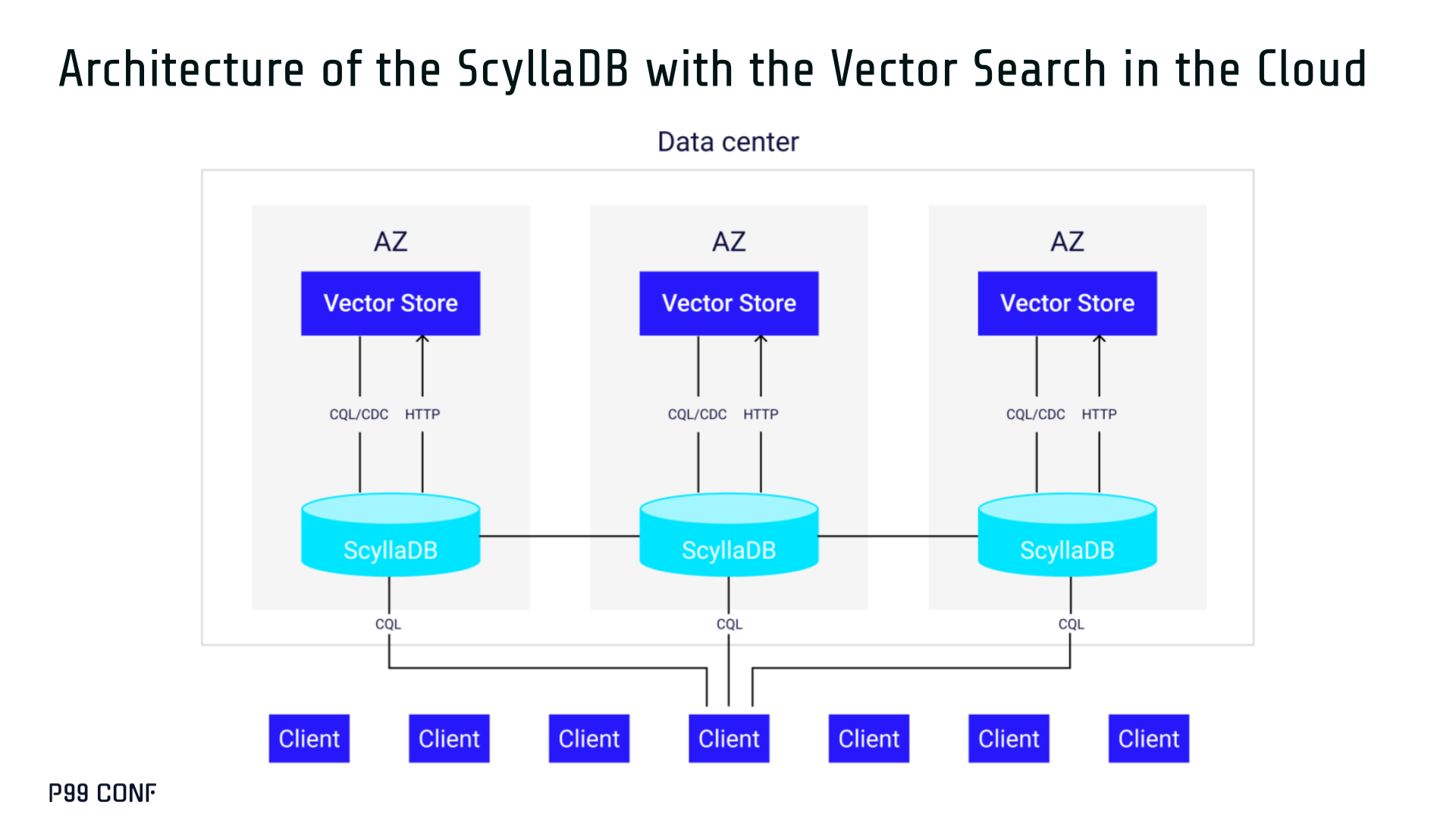
Inside the Database Internals Talks at P99 CONF 2025
“Never write a database. Even if you want to, even if you think you should. Resist. Never write a database. Unless you have to write a database. But you don’t.” – Charity MajorsBut someone has to write the databases that others rely on. Hearing about the engineering challenges they’re tackling is both fascinating and Schadenfreude-invoking – so perfect tech conference material. 😉 Since database performance is so near and dear to ScyllaDB, we reached out to our friends and colleagues across the community to that ensure a nice range of distributed data systems, approaches, and challenges would be represented at P99 CONF 2025. As you can see from our agenda, the response was overwhelming. A quick PSA for the uninitiated: P99 CONF is a free 2-day community event that’s intentionally virtual, highly interactive, and purely technical. It’s an immersion into all things performance. Distributed systems, database internals, Rust, C++, Java, Go, Wasm, Zig, Linux kernel, tracing, AI/ML & more – it’s all on the agenda. This year, you can look forward to first-hand engineering experiences from the likes of Pinterest, Clickhouse, Gemini, Arm, Rivian and VW Group Technology, Meta, Wayfair, Disney, NVIDIA, Turso, Neon, TigerBeetle, ScyllaDB, and too many others to list here. Here’s a sneak peek of the database internals talks you can look forward to at P99 CONF 2025… Join us at P99 CONF (free + virtual) Clickhouse’s C++ and Rust Journey Alexey Milovidov, Co-founder and CTO at Clickhouse Full rewrite from C++ to Rust or gradual integration with Rust libraries? For a large C++ codebase, only the latter works, but even then, there are many complications and rough edges. In my presentation, I will describe our experience integrating Rust and C++ code and some weird and unusual problems we had to overcome. Rethinking Durable Workflows and Queues: A Library-based Approach Qian Li, Co-founder at DBOS, Inc Durable workflow engines checkpoint program state to persistent storage (like a database) so that execution can always recover from where it left off. Most systems today rely on external orchestration: a centralized orchestrator and distributed workers communicating via message-passing. While this model is well-established, it’s often heavyweight, introducing substantial overhead, write amplification, and operational complexity. In this talk, we explore an alternative: a lightweight library-based durable workflow engine that embeds into application code and checkpoint state directly to the database. It handles queues and flow control through the database itself. This approach eliminates the need for a separate orchestrator, reduces network traffic, and improves performance by avoiding unnecessary writes. We’ll share our experience building DBOS, a library-based engine designed for simplicity and efficiency. We’ll discuss the architectural trade-offs, challenges in failure recovery, and key optimizations for scalability and maintainability. The Gory Details of a Full-Featured Userspace CPU Scheduler Avi Kivity, Co-founder and CTO at ScyllaDB Userspace CPU schedulers, which often accompany asynchronous I/O engines like io_uring and Linux AIO, are usually simplistic run-to-completion FIFO loops. This suffices for I/O bound applications, but for use cases that can be both CPU bound and I/O bound, this is not enough. Avi Kivity, CTO of ScyllaDB and co-maintainer of Seastar, will cover the design and implementation of the Seastar userspace CPU scheduler, which caters to more complex applications that require preemption and prioritization. The Tale of Taming TigerBeetle’s Tail Latency Tobias Ziegler, Software Engineer at Tigerbeetle In this talk, we dive into how we reduced TigerBeetle’s tail latency through algorithm engineering. ‘Algorithm engineering goes beyond studying theoretical complexity and considers how algorithms are executed efficiently on modern super-scalar CPUs. Specifically, we will look at Radix Sort and a k-way merge and explore how to implement them efficiently. We then demonstrate how we apply these algorithms incrementally to avoid latency spikes in practice. Why We’re Rewriting SQLite in Rust Glauber Costa, Co-founder and CEO at Turso Over two years ago, we forked SQLite. We were huge fans of the embedded nature of SQLite, but wanted a more open model of development…and libSQL was born as an Open Contribution project. Last year, as we were adding Vector Search to SQLite, we had a crazy idea. What could we achieve if we were to completely rewrite SQLite in Rust? This talk explains what drove us down this path, how we’re using deterministic simulation testing to ensure the reliability of the Rust rewrite, and the lessons learned (so far). I will show how a reimagining of this iconic database can lead to performance improvements of over 500x in some cases by looking at what powers it under the hood. Shared Nothing Databases at Scale Nick Van Wiggeren, CTO at PlanetScale This talk will discuss how PlanetScale scales databases in the cloud, focusing on a shared-nothing architecture that is built around expecting failure. Nick will go into how they built low-latency high-throughput systems that span multiple nodes, availability zones, and regions, while maintaining sub-millisecond response times. This starts at the storage layer and builds all the way up to micro-optimizing the load balancer, with a lot of learning at every step of the way. Reworking the Neon IO stack: Rust+tokio+io_uring+O_DIRECT Christian Schwarz, Member of Technical Staff at Databricks Neon is a serverless Postgres platform. Recently acquired by Databricks, the same technology now also powers Databricks Lakebase. In this talk, we will dive into Pageserver, the multi-tenant storage service at the heart of the architecture. We share techniques and lessons learned from reworking its IO stack to a fully asynchronous model, with direct IO against local NVMe drives; all during a period of rapid growth. Pageserver is implemented in Rust, we use the tokio async runtime for networking, and integrate it with io_uring for filesystem access. A Deep Dive into the Seastar Event Loop Pavel Emelyanov, Principal Software Engineer at ScyllaDB The core and the basis of ScyllaDB’s outstanding performance is the Seastar framework, and the core and the basis of seastar is its event loop. In this presentation, we’ll see what the loop does in great detail, analyze the limitations that it runs in and all the consequences that follow those limitations. We’ll also learn how the loop is observed by the user and various means to understand its behavior. Cost Effective, Low Latency Vector Search In Databases: A Case Study with Azure Cosmos DB Magdalen Manohar, Senior Researcher at Microsoft We’ve integrated DiskANN, a state-of-the-art vector indexing algorithm, into Azure Cosmos DB NoSQL, a state-of-the-art cloud-native operational database. Learn how we overcame the systems and algorithmic challenges of this integration to achieve <20ms query latency at the 10 million scale, while supporting scale-out to billions of vectors via automatic partitioning. Measuring Query Latency the Hard Way: An Adventure in Impractical Postgres Monitoring Simon Notley, Observability and Optimization at EnterpriseDB Sampling the session state (as exposed by pg_stat_activity) is a surprisingly powerful way to understand how your Postgres instance spends its time. It is something I can wholeheartedly recommend to any Postgres DBA that needs a lightweight way to monitor query performance in production. However, it’s a terrible way to measure query latency, fraught with complexity and weird statistical biases that could be avoided by simply using an extension built for the job, or even log analysis. But pursuing terrible ideas can be fun, so in this talk, I dive into my adventures in measuring query latency from session sampling, generate some extremely funky charts, and end up unexpectedly performing a vector similarity search. In this talk I’ll show how instead of attempting to correct the biases that plague estimates of query latency based time-domain sampling, we can instead pre-calculate the distribution of (biased) estimates based on a range of true distributions and use vector search to compare our observed distribution to these pre-calculate ones, thereby inferring the true query latency. This ‘eccentric’ method is actually surprisingly effective, and surprisingly fun. Fast and Deterministic Full Table Scans at Scale Felipe Cardeneti Mendes, Technical Director at ScyllaDB ScyllaDB’s new tablet replication algorithm replaces static vNodes with dynamic, elastic data distribution that adapts to shifting workloads. This talk discusses how tablets enable fast, predictable full table scans by keeping operations shard-local, balancing load automatically, and scaling linearly through a simple layer of indirection. Optimizing Tiered Storage for Low-Latency Real-Time Analytics Neha Pawar, Founding Engineer and Head of Data at StarTree Real-time OLAP databases usually trade performance for cost when moving from local storage to cloud object storage. This talk shows how we extended Apache Pinot to use cloud storage while still achieving sub-second P99 latencies. We’ll cover the abstraction that makes Pinot location-agnostic, strategies like pipelining, prefetching, and selective block fetches, and how to balance local and cloud storage for both cost efficiency and speed. As Fast as Possible, But Not Faster: ScyllaDB Flow Control Nadav Har’El, Distinguished Engineer at ScyllaDB Pushing requests faster than a system can handle results in rapidly growing queues. If unchecked, it risks depleting memory and system stability. This talk discusses how we engineered ScyllaDB’s flow control for high volume ingestions, allowing it to throttle over-eager clients to exactly the right pace – not so fast that we run out of memory, but also not so slow that we let available resources go to waste. Push the Database Beyond the Edge Nikita Sivukhin, Software Engineer at Turso Almost any application can benefit from having data available locally – enabling blazing-fast access and optimized write patterns. This talk will walk you through one approach to designing a full-featured sync engine, applicable across a wide range of domains, including front-end, back-end, and machine learning training. Engineering a Low-Latency Vector Search Engine for ScyllaDB Pawel Pery, Senior Software Engineer at ScyllaDB Implementing Vector Search in ScyllaDB brings challenges from low-latency to predictable performance at scale. Rather than embedding HNSW indexing directly into the core database, we decoupled vector indexing and similarity search into a dedicated Rust engine. Learn about the architectural design decisions that enabled us to combine and integrate ScyllaDB’s shard-per-core for real-time operations and high-performance ANN processing via USearch. We Told B+ Trees to Do Sorted Sets—They Nailed It (Joe Zhou, Dragonfly) Joe Zhou, Developer Advocate at DragonflyDB Sorted sets are a critical Redis data type used for leaderboards, time-series data, and priority queues. However, Redis’s skiplist-based implementation introduces significant memory overhead—averaging 37 bytes per entry on top of the essential 16 bytes for the (member, score) pair. For large sorted sets, this inefficiency can become a major bottleneck. In this talk, we’ll explore how Dragonfly reimplemented sorted sets using a B+ tree, reducing memory overhead to just 2-3 bytes per entry while improving performance. We’ll cover: Why skiplists are inefficient for large sorted sets. How B+ trees with bucketing drastically cut memory usage while maintaining O(log N) operations. Benchmark results showing 40% lower memory and better throughput vs. Redis. This optimization, now stable in Dragonfly, demonstrates how rethinking core data structures can unlock major efficiency gains. Attendees will leave with insights into: Trade-offs between skiplists and B+ trees. Real-world impact on memory and latency (P99 improvements). Lessons from implementing a custom ranking API for B+ trees. Keynote: Andy Pavlo You can also look forward to a keynote by Andy Pavlo. We’re not revealing the topic yet, but if you know Andy, you know you won’t want to miss it. Join us at P99 CONF (free + virtual)
Building a Resilient Data Platform with Write-Ahead Log at Netflix
By Prudhviraj Karumanchi, Samuel Fu, Sriram Rangarajan, Vidhya Arvind, Yun Wang, John Lu
Introduction
Netflix operates at a massive scale, serving hundreds of millions of users with diverse content and features. Behind the scenes, ensuring data consistency, reliability, and efficient operations across various services presents a continuous challenge. At the heart of many critical functions lies the concept of a Write-Ahead Log (WAL) abstraction. At Netflix scale, every challenge gets amplified. Some of the key challenges we encountered include:
- Accidental data loss and data corruption in databases
- System entropy across different datastores (e.g., writing to Cassandra and Elasticsearch)
- Handling updates to multiple partitions (e.g., building secondary indices on top of a NoSQL database)
- Data replication (in-region and across regions)
- Reliable retry mechanisms for real time data pipeline at scale
- Bulk deletes to database causing OOM on the Key-Value nodes
All the above challenges either resulted in production incidents or outages, consumed significant engineering resources, or led to bespoke solutions and technical debt. During one particular incident, a developer issued an ALTER TABLE command that led to data corruption. Fortunately, the data was fronted by a cache, so the ability to extend cache TTL quickly together with the app writing the mutations to Kafka allowed us to recover. Absent the resilience features on the application, there would have been permanent data loss. As the data platform team, we needed to provide resilience and guarantees to protect not just this application, but all the critical applications we have at Netflix.
Regarding the retry mechanisms for real time data pipelines, Netflix operates at a massive scale where failures (network errors, downstream service outages, etc.) are inevitable. We needed a reliable and scalable way to retry failed messages, without sacrificing throughput.
With these problems in mind, we decided to build a system that would solve all the aforementioned issues and continue to serve the future needs of Netflix in the online data platform space. Our Write-Ahead Log (WAL) is a distributed system that captures data changes, provides strong durability guarantees, and reliably delivers these changes to downstream consumers. This blog post dives into how Netflix is building a generic WAL solution to address common data challenges, enhance developer efficiency, and power high-leverage capabilities like secondary indices, enable cross-region replication for non-replicated storage engines, and support widely used patterns like delayed queues.
API
Our API is intentionally simple, exposing just the essential parameters. WAL has one main API endpoint, WriteToLog, abstracting away the internal implementation and ensuring that users can onboard easily.
rpc WriteToLog (WriteToLogRequest) returns (WriteToLogResponse) {...}

/**
  * WAL request message
  * namespace: Identifier for a particular WAL
  * lifecycle: How much delay to set and original write time
  * payload: Payload of the message
  * target: Details of where to send the payload
  */
message WriteToLogRequest {
  string namespace = 1;
  Lifecycle lifecycle = 2;
  bytes payload = 3;
  Target target = 4;
}

/**
  * WAL response message
  * durable: Whether the request succeeded, failed, or unknown
  * message: Reason for failure
  */
message WriteToLogResponse {
  Trilean durable = 1;
  string message = 2;
}
A namespace defines where and how data is stored, providing logical separation while abstracting the underlying storage systems. Each namespace can be configured to use different queues: Kafka, SQS, or combinations of multiple. Namespace also serves as a central configuration of settings, such as backoff multiplier or maximum number of retry attempts, and more. This flexibility allows our Data Platform to route different use cases to the most suitable storage system based on performance, durability, and consistency needs.
WAL can assume different personas depending on the namespace configuration.
Persona #1 (Delayed Queues)
In the example configuration below, the Product Data Systems (PDS) namespace uses SQS as the underlying message queue, enabling delayed messages. PDS uses Kafka extensively, and failures (network errors, downstream service outages, etc.) are inevitable. We needed a reliable and scalable way to retry failed messages, without sacrificing throughput. That’s when PDS started leveraging WAL for delayed messages.
"persistenceConfigurations": {
  "persistenceConfiguration": [
  {
    "physicalStorage": {
      "type": "SQS",
    },
    "config": {
      "wal-queue": [
        "dgwwal-dq-pds"
      ],
      "wal-dlq-queue": [
        "dgwwal-dlq-pds"
      ],
      "queue.poll-interval.secs": 10,
      "queue.max-messages-per-poll": 100
    }
  }
  ]
}
Persona #2 (Generic Cross-Region Replication)
Below is the namespace configuration for cross-region replication of EVCache using WAL, which replicates messages from a source region to multiple destinations. It uses Kafka under the hood.
"persistence_configurations": {
  "persistence_configuration": [
  {
    "physical_storage": {
      "type": "KAFKA"
    },
    "config": {
      "consumer_stack": "consumer",
      "context": "This is for cross region replication for evcache_foobar",
      "target": {
        "euwest1": "dgwwal.foobar.cluster.eu-west-1.netflix.net",
        "type": "evc-replication",
        "useast1": "dgwwal.foobar.cluster.us-east-1.netflix.net",
        "useast2": "dgwwal.foobar.cluster.us-east-2.netflix.net",
        "uswest2": "dgwwal.foobar.cluster.us-west-2.netflix.net"
      },
      "wal-kafka-dlq-topics": [],
      "wal-kafka-topics": [
        "evcache_foobar"
      ],
      "wal.kafka.bootstrap.servers.prefix": "kafka-foobar"
    }
  }
  ]
}
Persona #3 (Handling multi-partition mutations)
Below is the namespace configuration for supporting mutateItems API in Key-Value, where multiple write requests can go to different partitions and have to be eventually consistent. A key detail in the below configuration is the presence of Kafka and durable_storage. These data stores are required to facilitate two phase commit semantics, which we will discuss in detail below.
"persistence_configurations": {
  "persistence_configuration": [
  {
    "physical_storage": {
      "type": "KAFKA"
    },
    "config": {
      "consumer_stack": "consumer",
      "contacts": "unknown",
      "context": "WAL to support multi-id/namespace mutations for dgwkv.foobar",
      "durable_storage": {
        "namespace": "foobar_wal_type",
        "shard": "walfoobar",
        "type": "kv"
      },
      "target": {},
      "wal-kafka-dlq-topics": [
        "foobar_kv_multi_id-dlq"
      ],
      "wal-kafka-topics": [
        "foobar_kv_multi_id"
      ],
      "wal.kafka.bootstrap.servers.prefix": "kaas_kafka-dgwwal_foobar7102"
    }
  }
  ]
}
An important note is that requests to WAL support at-least once semantics due to the underlying implementation.
Under the Hood
The core architecture consists of several key components working together.
Message Producer and Message Consumer separation: The message producer receives incoming messages from client applications and adds them into the queue, while the message consumer processes messages from the queue and sends them to the targets. Because of this separation, other systems can bring their own pluggable producers or consumers, depending on their use cases. WAL’s control plane allows for a pluggable model, which, depending on the use-case, allows us to switch between different message queues.
SQS and Kafka with a dead letter queue by default: Every WAL namespace has its own message queue and gets a dead letter queue (DLQ) by default, because there can be transient errors and hard errors. Application teams using Key-Value abstraction simply need to toggle a flag to enable WAL and get all this functionality without needing to understand the underlying complexity.
- Kafka-backed namespaces: handle standard message processing
- SQS-backed namespaces: support delayed queue semantics (we added custom logic to go beyond the standard defaults enforced in terms of delay, size limits, etc)
- Complex multi-partition scenarios: use queues and durable storage
Target Flexibility: The messages added to WAL are pushed to the target datastores. Targets can be Cassandra databases, Memcached caches, Kafka queues, or upstream applications. Users can specify the target via namespace configuration and in the API itself.

Deployment Model
WAL is deployed using the Data Gateway infrastructure. This means that WAL deployments automatically come with mTLS, connection management, authentication, runtime and deployment configurations out of the box.
Each data gateway abstraction (including WAL) is deployed as a shard. A shard is a physical concept describing a group of hardware instances. Each use case of WAL is usually deployed as a separate shard. For example, the Ads Events service will send requests to WAL shard A, while the Gaming Catalog service will send requests to WAL shard B, allowing for separation of concerns and avoiding noisy neighbour problems.
Each shard of WAL can have multiple namespaces. A namespace is a logical concept describing a configuration. Each request to WAL has to specify its namespace so that WAL can apply the correct configuration to the request. Each namespace has its own configuration of queues to ensure isolation per use case. If the underlying queue of a WAL namespace becomes the bottleneck of throughput, the operators can choose to add more queues on the fly by modifying the namespace configurations. The concept of shards and namespaces is shared across all Data Gateway Abstractions, including Key-Value, Counter, Timeseries, etc. The namespace configurations are stored in a globally replicated Relational SQL database to ensure availability and consistency.

Based on certain CPU and network thresholds, the Producer group and the Consumer group of each shard will (separately) automatically scale up the number of instances to ensure the service has low latency, high throughput and high availability. WAL, along with other abstractions, also uses the Netflix adaptive load shedding libraries and Envoy to automatically shed requests beyond a certain limit. WAL can be deployed to multiple regions, so each region will deploy its own group of instances.
Solving different flavors of problems with no change to the core architecture
The WAL addresses multiple data reliability challenges with no changes to the core architecture:
Data Loss Prevention: In case of database downtime, WAL can continue to hold the incoming mutations. When the database becomes available again, replay mutations back to the database. The tradeoff is eventual consistency rather than immediate consistency, and no data loss.
Generic Data Replication: For systems like EVCache (using Memcached) and RocksDB that do not support replication by default, WAL provides systematic replication (both in-region and across-region). The target can be another application, another WAL, or another queue — it’s completely pluggable through configuration.
System Entropy and Multi-Partition Solutions: Whether dealing with writes across two databases (like Cassandra and Elasticsearch) or mutations across multiple partitions in one database, the solution is the same — write to WAL first, then let the WAL consumer handle the mutations. No more asynchronous repairs needed; WAL handles retries and backoff automatically.
Data Corruption Recovery: In case of DB corruptions, restore to the last known good backup, then replay mutations from WAL omitting the offending write/mutation.
There are some major differences between using WAL and directly using Kafka/SQS. WAL is an abstraction on the underlying queues, so the underlying technology can be swapped out depending on use cases with no code changes. WAL emphasizes an easy yet effective API that saves users from complicated setups and configurations. We leverage the control plane to pivot technologies behind WAL when needed without app or client intervention.
WAL usage at Netflix
Delay Queue
The most common use case for WAL is as a Delay Queue. If an application is interested in sending a request at a certain time in the future, it can offload its requests to WAL, which guarantees that their requests will land after the specified delay.
Netflix’s Live Origin processes and delivers Netflix live stream video chunks, storing its video data in a Key-Value abstraction backed by Cassandra and EVCache. When Live Origin decides to delete certain video data after an event is completed, it issues delete requests to the Key-Value abstraction. However, the large amount of delete requests in a short burst interfere with the more important real-time read/write requests, causing performance issues in Cassandra and timeouts for the incoming live traffic. To get around this, Key-Value issues the delete requests to WAL first, with a random delay and jitter set for each delete request. WAL, after the delay, sends the delete requests back to Key-Value. Since the deletes are now a flatter curve of requests over time, Key-Value is then able to send the requests to the datastore with no issues.

Additionally, WAL is used by many services that utilize Kafka to stream events, including Ads, Gaming, Product Data Systems, etc. Whenever Kafka requests fail for any reason, the client apps will send WAL a request to retry the kafka request with a delay. This abstracts away the backoff and retry layer of Kafka for many teams, increasing developer efficiency.


Cross-Region Replication
WAL is also used for global cross-region replication. The architecture of WAL is generic and allows any datastore/applications to onboard for cross-region replication. Currently, the largest use case is EVCache, and we are working to onboard other storage engines.
EVCache is deployed by clusters of Memcached instances across multiple regions, where each cluster in each region shares the same data. Each region’s client apps will write, read, or delete data from the EVCache cluster of the same region. To ensure global consistency, the EVCache client of one region will replicate write and delete requests to all other regions. To implement this, the EVCache client that originated the request will send the request to a WAL corresponding to the EVCache cluster and region.
Since the EVCache client acts as the message producer group in this case, WAL only needs to deploy the message consumer groups. From there, the multiple message consumers are set up to each target region. They will read from the Kafka topic, and send the replicated write or delete requests to a Writer group in their target region. The Writer group will then go ahead and replicate the request to the EVCache server in the same region.

The biggest benefits of this approach, compared to our legacy architecture, is being able to migrate from multi-tenant architecture to single tenant architecture for the most latency sensitive applications. For example, Live Origin will have its own dedicated Message Consumer and Writer groups, while a less latency sensitive service can be multi-tenant. This helps us reduce the blast radius of the issues and also prevents noisy neighbor issues.
Multi-Table Mutations
WAL is used by Key-Value service to build the MutateItems API. WAL enables the API’s multi-table and multi-id mutations by implementing 2-phase commit semantics under the hood. For this discussion, we can assume that Key-Value service is backed by Cassandra, and each of its namespaces represents a certain table in a Cassandra DB.
When a Key-Value client issues a MutateItems request to Key-Value server, the request can contain multiple PutItems or DeleteItems requests. Each of those requests can go to different ids and namespaces, or Cassandra tables.
message MutateItemsRequest {
 repeated MutationRequest mutations = 1;
 message MutationRequest {
  oneof mutation {
    PutItemsRequest put = 1;
    DeleteItemsRequest delete = 2;
  }
 }
}
The MutateItems request operates on an eventually consistent model. When the Key-Value server returns a success response, it guarantees that every operation within the MutateItemsRequest will eventually complete successfully. Individual put or delete operations may be partitioned into smaller chunks based on request size, meaning a single operation could spawn multiple chunk requests that must be processed in a specific sequence.
Two approaches exist to ensure Key-Value client requests achieve success. The synchronous approach involves client-side retries until all mutations complete. However, this method introduces significant challenges; datastores might not natively support transactions and provide no guarantees about the entire request succeeding. Additionally, when more than one replica set is involved in a request, latency occurs in unexpected ways, and the entire request chain must be retried. Also, partial failures in synchronous processing can leave the database in an inconsistent state if some mutations succeed while others fail, requiring complex rollback mechanisms or leaving data integrity compromised. The asynchronous approach was ultimately adopted to address these performance and consistency concerns.
Given Key-Value’s stateless architecture, the service cannot maintain the mutation success state or guarantee order internally. Instead, it leverages a Write-Ahead Log (WAL) to guarantee mutation completion. For each MutateItems request, Key-Value forwards individual put or delete operations to WAL as they arrive, with each operation tagged with a sequence number to preserve ordering. After transmitting all mutations, Key-Value sends a completion marker indicating the full request has been submitted.
The WAL producer receives these messages and persists the content, state, and ordering information to a durable storage. The message producer then forwards only the completion marker to the message queue. The message consumer retrieves these markers from the queue and reconstructs the complete mutation set by reading the stored state and content data, ordering operations according to their designated sequence. Failed mutations trigger re-queuing of the completion marker for subsequent retry attempts.


Closing Thoughts
Building Netflix’s generic Write-Ahead Log system has taught us several key lessons that guided our design decisions:
Pluggable Architecture is Core: The ability to support different targets, whether databases, caches, queues, or upstream applications, through configuration rather than code changes has been fundamental to WAL’s success across diverse use cases.
Leverage Existing Building Blocks: We had control plane infrastructure, Key-Value abstractions, and other components already in place. Building on top of these existing abstractions allowed us to focus on the unique challenges WAL needed to solve.
Separation of Concerns Enables Scale: By separating message processing from consumption and allowing independent scaling of each component, we can handle traffic surges and failures more gracefully.
Systems Fail — Consider Tradeoffs Carefully: WAL itself has failure modes, including traffic surges, slow consumers, and non-transient errors. We use abstractions and operational strategies like data partitioning and backpressure signals to handle these, but the tradeoffs must be understood.
Future work
- We are planning to add secondary indices in Key-Value service leveraging WAL.
- WAL can also be used by a service to guarantee sending requests to multiple datastores. For example, a database and a backup, or a database and a queue at the same time etc.
Acknowledgements
Launching WAL was a collaborative effort involving multiple teams at Netflix, and we are grateful to everyone who contributed to making this idea a reality. We would like to thank the following teams for their roles in this launch.
- Caching team — Additional thanks to Shih-Hao Yeh, Akashdeep Goel for contributing to cross region replication for KV, EVCache etc. and owning this service.
- Product Data System team — Carlos Matias Herrero, Brandon Bremen for contributing to the delay queue design and being early adopters of WAL giving valuable feedback.
- KeyValue and Composite abstractions team — Raj Ummadisetty for feedback on API design and mutateItems design discussions. Rajiv Shringi for feedback on API design.
- Kafka and Real Time Data Infrastructure teams — Nick Mahilani for feedback and inputs on integrating the WAL client into Kafka client. Sundaram Ananthanarayan for design discussions around the possibility of leveraging Flink for some of the WAL use cases.
- Joseph Lynch for providing strategic direction and organizational support for this project.
Building a Resilient Data Platform with Write-Ahead Log at Netflix was originally published in Netflix TechBlog on Medium, where people are continuing the conversation by highlighting and responding to this story.
ScyllaDB X Cloud: An Inside Look with Avi Kivity (Part 3)
ScyllaDB’s co-founder/CTO discusses decisions to increase efficiency for storage-bound workloads and allow deployment on mixed size clusters To get the engineering perspective on the recent shifts to ScyllaDB’s architecture, Tim Koopmans recently caught up with ScyllaDB Co-Founder and CTO Avi Kivity. In part 1 of this 3-part series, they talked about the motivations and architectural shifts behind ScyllaDB X Cloud, particularly with respect to Raft and tablets-based data distribution. In part 2, they went deeper into how tablets work, then looked at the design of ScyllaDB X Cloud’s autoscaling. In this final part of the series, they discuss changes that increase efficiency for storage-bound workloads and allow deployment on mixed size clusters. You can watch the complete video here. Storage-bound workloads and compression Tim: Let’s switch gears and talk about compression. This was a way to double-down on storage-bound workloads, right? Would you say storage-bound workloads are more common than CPU bound ones? Is that what’s driving this? Avi: Yes, and there’s two reasons for that. One reason is that our CPU efficiency is quite high. If you’re CPU-efficient, then storage is going to dominate. And the other reason is that when your database grows – say it’s twice as large as before – it’s rare that you actually have twice the amount of work. It can happen. But for many workloads, the growth of data is mostly historical, so the number of ops doesn’t scale linearly with the size of the database. As the database grows, the ratio of ops to storage decreases, and it becomes storage-bound. So, many of our larger workloads are storage-bound. The small and medium ones can be either storage-bound or CPU-bound…it really depends on the workload. We have some workloads where most of the storage in the cluster isn’t used because they’re so CPU-intensive. And we have others where the CPU is mostly idle, but the cluster is holding a lot of storage. We try to cater to all of these workloads. Tim: So a storage-bound workload is likely to have lower CPU utilization in general, and that gives you more CPU bandwidth to do things like more advanced compression? What’s the default compression, in terms of planning for storage? Is it like 50%? Or what’s the typical rate? Or is the real answer just “it depends”? Avi: “It depends” is an easy escape, but the truth is there’s a wide variety of storage options now. A recent addition is dictionary-based compression. That’s where the cluster periodically samples data on disk and constructs a dictionary from those samples. That dictionary is then used to boost compression. Everyone probably knows dictionary compression: it finds repetitive byte sequences in the data and matches against them. By having samples, you can match against the samples and gain higher compression. We recently started rolling it out, and it does give a nice improvement. Of course, it varies widely. Some people store data that’s already compressed, so it won’t compress further. Others store data like JSON, which compresses very well. In those cases, we might see above 50% compression ratios. And for many storage-bound workloads, you can set the compression parameters higher and gain more compression at the expense of CPU…but it’s CPU that you already have. Tim: Is there anything else on the compression roadmap, like column aware compression? Avi: It’s not on the roadmap yet, but we will do columnar storage for time series and data. But there’s no timeline for that yet. Tim: Any hardware accelerated stuff? Avi: We looked at hardware acceleration, but it’s too rare to really matter. One problem is that on the cloud, it’s only available with the very largest instance sizes. And while we do have clusters with large instance sizes, it’s not enough to justify the work. I’m talking about machines with 96 vCPUs and 60TB of storage per node. It would only make sense for the very largest clusters, the petabyte-class clusters. They do exist, but they’re not yet common enough to make it worth the effort. On smaller instances, the accelerators are just hidden by virtualization. The other problem with hardware-accelerated compression is that it doesn’t keep up with the advances in software compression. That’s a general problem with hardware. For example, dictionary compression isn’t supported by those accelerators, but dictionary compression is very useful. We wouldn’t want to give that up. Tim: Yeah, it seems like unless there’s a very specific, almost niche need for it, it’s safer to stick with software-based compression. Mixed size types & CPU: Storage ratios Tim: And in a roundabout way, this brings me back to the last thing I wanted to ask about. I think we’ve already touched on it: the idea of 90% storage utilization. You’ve already mentioned reasons why, including tablets. And we also spoke about having mixed instance types in the cluster. That’s quite significant for this release, right? Avi: Yes, it’s quite important. Assume you have those large instances with 96 vCPUs and 60TB of storage per node… and your data grows. It’s not doubling, just incremental growth. If you have a large amount of data, the rate of growth won’t be very large. So, you want to add a smaller amount of storage each time, not 60TB. That gives you two options. One option is to compose your cluster from a large number of very small instances. But large clusters introduce management problems. The odds of a node failing grow as the cluster grows, so you want to keep clusters at a manageable size. The other option is to have mixed-size clusters. For example, if you have clusters of 60TB nodes, then you might add a 6TB node. As the data grows, you can then replace those smaller nodes with larger ones, until you’re back to having a cluster that’s full of the largest node size. There’s another reason for mixed-size clusters: changing the CPU-to-storage ratio. Typically, storage bound clusters use nodes with a large disk-to-CPU ratio – a lot of disk and relatively little CPU. But there might be times across a day or throughout the year where the number of OPS increases without a corresponding increase in storage. For example, think about Black Friday or workloads spiking in certain geographies. In those cases, you might switch from nodes with a low CPU-to-disk ratio to ones with a high CPU-to-disk ratio, then switch back later. That way, you keep total storage constant, but increase the amount of CPU serving that storage. It lets you adapt to changing CPU requirements without having to buy more storage. Tim: Got it. So it’s really about averaging out the ratios to get the price–performance balance you want between storage and CPU. Is that something the user has to figure out, or does it fall under the autoscaler? Avi: It will be automatic. It’s too much to ask a user to track the right mix of instances and keep managing that. Looking back and looking forward Tim: Looking back, and a little forward…if you could go back to 2014, when you first came up with ScyllaDB, would you tell your past self to do anything different? Or do you think it’s evolved naturally? Would you save yourself some pain? Avi: Yeah. So, when you start a project, it always looks simple and you think you know everything. Then you discover how much you didn’t know. I don’t even know what my 2014 self would say about how much I mispredicted the amount of work that would be necessary to do this. I mean, I knew databases were hard – one of the most complex areas in software engineering – but I didn’t know how hard. Tim: And what about looking forward?What’s the next big thing on the horizon that people aren’t really talking about yet? Avi: I want to fully complete the tablets project before we talk about the next step. Tim: Just one last question from me before we wrap. Aside from the correct pronunciation of ScyllaDB, what’s the most misunderstood part of ScyllaDB’s new architecture? What are people getting wrong? Avi: I don’t think people are getting it wrong. It’s not that complicated. It’s another layer of indirection, and people do understand that. We have some nice visualizations of that as well. Maybe we should have a session showing how tablets move around, because it’s a little like Tetris – how we fit different tablets to fill the nodes. So I think tablets are easily understood. It’s complex to implement, but not complicated to understand.The Latency vs. Complexity Tradeoffs with 6 Caching Strategies
How to choose between cache-aside, read-through, write-through, client-side, and distributed caching strategies As we mentioned in the recent Why Cache Data? post, we’re delighted that Pekka Enberg decided to write an entire book on latency and we’re proud to sponsor 3 chapters from it. Get the Latency book excerpt PDF Also, Pekka just shared key takeaways from that book in a masterclass on Building Low Latency Apps (now available on demand). Let’s continue our Latency book excerpts with more from Pekka’s caching chapter. It’s reprinted here with permission of the publisher. *** When adding caching to your application, you must first consider your caching strategy, which determines how reads and writes happen from the cache and the underlying backing store, such as a database or a service. At a high level, you need to decide if the cache is passive or active when there is a cache miss. In other words, when your application looks up a value from the cache, but the value is not there or has expired, the caching strategy mandates whether it’s your application or the cache that retrieves the value from the backing store. As usual, different caching strategies have different trade-offs on latency and complexity, so let’s get right into it. Cache-Aside Caching Cache-aside caching is perhaps the most typical caching strategy you will encounter. When there is a cache hit, data access latency is dominated by communication latency, which is typically small, as you can get a cache close by on a cache server or even in your application memory space. However, when there is a cache miss, with cache-aside caching, the cache is a passive store updated by the application. That is, the cache just reports a miss and the application is responsible for fetching data from the backing store and updating the cache. Figure 1 shows an example of cache-aside caching in action. An application looks up a value from a cache by a caching key, which determines the data the application is interested in. If the key exists in the cache, the cache returns the value associated with the key, which the application can use. However, if the key does not exist or is expired in the cache, we have a cache miss, which the application has to handle. The application queries the value from the backing store and stores the value in the cache. Suppose you are caching user information and using the user ID as the lookup key. In that case, the application performs a query by the user ID to read user information from the database. The user information returned from the database is then transformed into a format you can store in the cache. Then, the cache is updated with the user ID as the cache key and the information as the value. For example, a typical way to perform this type of caching is to transform the user information returned from the database into JSON and store that in the cache. Figure 1: With cache-aside caching, the client first looks up a key from the cache. On cache miss, the client queries the database and updates the cache. Cache-aside caching is popular because it is easy to set up a cache server such as Redis and use it to cache database queries and service responses. With cache-aside caching, the cache server is passive and does not need to know which database you use or how the results are mapped to the cache. It is your application doing all the cache management and data transformation. In many cases, cache-aside caching is a simple and effective way to reduce application latency. You can hide database access latency by having the most relevant information in a cache server close to your application. However, cache-aside caching can also be problematic if you have data consistency or freshness requirements. For example, if you have multiple concurrent readers that are looking up a key in the cache, you need to coordinate in your application how you handle concurrent cache misses; otherwise, you may end up with multiple database accesses and cache updates, which may result in subsequent cache lookups returning different values. However, with cache-aside caching, you lose transaction support because the cache and the database do not know each other, and it’s the application’s responsibility to coordinate updates to the data. Finally, cache-aside caching can have significant tail latency because some cache lookups experience the database read latency on a cache miss. That is, although in the case of a cache hit, access latency is fast because it’s coming from a nearby cache server; cache lookups that experience a cache miss are only as fast as database access. That’s why the geographic latency to your database still can matter a great deal even if you are caching because tail latency is experienced surprisingly often in many scenarios. Read-Through Caching Read-through caching is a strategy where, unlike cache-aside caching, the cache is an active component when there is a cache miss. When there is a cache miss, a read-through cache attempts to read a value for the key from the backing store automatically. Latency is similar to cache-aside caching, although backing store retrieval latency is from the cache to the backing store, not from application to backing store, which may be smaller, depending on your deployment architecture. Figure 2 shows an example of a read-through cache in action. The application performs a cache lookup on a key, and if there is a cache miss, the cache performs a read to the database to obtain the value for the key. The cache then updates itself and returns the value to the application. From an application point of view, a cache miss is transparent because the cache always returns a key if one exists, regardless of whether there was a cache miss or not. Figure 2: With read-through caching, the client looks up a key from the cache. Unlike with cache-aside caching, the cache queries the database and updates itself on cache miss. Read-through caching is more complex to implement because a cache needs to be able to read the backing store, but it also needs to transform the database results into a format for the cache. For example, if the backing store is an SQL database server, you need to convert the query results into a JSON or similar format to store the results in the cache. The cache is, therefore, more coupled with your application logic because it needs to know more about your data model and formats. However, because the cache coordinates the updates and the database reads with read-through caching, it can give transactional guarantees to the application and ensure consistency on concurrent cache misses. Furthermore, although a read-through cache is more complex from an application integration point of view, it does remove cache management complexity from the application. Of course, the same caveat of tail latency applies to read-through caches as they do to cache-aside caching. An exception: as active components, read-through caches can hide the latency better with, for example, refresh-ahead caching. Here, the cache asynchronously updates the cache before the values are expired – therefore hiding the database access latency from applications altogether when a value is in the cache. Write-Through Caching Cache-aside and read-through caching are strategies around caching reads, but sometimes, you also want the cache to support writes. In such cases, the cache provides an interface for updating the value of a key that the application can invoke. In the case of cache-aside caching, the application is the only one communicating with the backing store and, therefore, updates the cache. However, with read-through caching, there are two options for dealing with writes: write-through and write-behind caching. Write-through caching is a strategy where an update to the cache propagates immediately to the backing store. Whenever a cache is updated, the cache synchronously updates the backing store with the cached value. The write latency of write-through cache is dominated by the write latency to the backing store, which can be significant. As shown in Figure 3, an application updates a cache using an interface provided by the cache with a key and a value pair. The cache updates its state with the new value, updates the database with the new value and waits for the database to commit the update until acknowledging the cache update to the application. Figure 3: With write-through caching, the client writes a key-value pair to the cache. The cache immediately updates the cache and the database. Write-through caching aims to keep the cache and the backing storage in sync. However, for non-transactional caches, the cache and backing store can be out of sync in the presence of errors. For example, if write to cache succeeds, but the write to backing store fails, the two will be out of sync. Of course, a write-through cache can provide transactional guarantees by trading off some latency to ensure that the cache and the database are either both updated or neither of them is. As with a read-through cache, write-through caching assumes that the cache can connect to the database and transform a cache value into a database query. For example, if you are caching user data where the user ID serves as the key and a JSON document represents the value, the cache must be able to transform the JSON representation of user information into a database update. With write-through caching, the simplest solution is often to store the JSON in the database. The primary drawback of write-through caching is the latency associated with cache updates, which is essentially equivalent to database commit latency. This can be significant. Write-Behind Caching Write-behind caching strategy updates the cache immediately, unlike write-through caching, which defers the database updates. In other words, with write-behind caching, the cache may accept multiple updates before updating the backing store, as shown in Figure 4, where the cache accepts three cache updates before updating the database. Figure 4: With write-behind caching, the client writes a key-value pair to the cache. However, unlike with write-through caching, the cache updates the cache but defers the database update. Instead, write-behind cache will batch multiple cache updates to a single database update. The write latency of a write-behind cache is lower than with write-through caching because the backing store is updated asynchronously. That is, the cache can acknowledge the write immediately to the application, resulting in a low-latency write, and then perform the backing store update in the background. However, the downside of write-behind caching is that you lose transaction support because the cache can no longer guarantee that the cache and the database are in sync. Furthermore, write-behind caching can reduce durability, which is the guarantee that you don’t lose data. If the cache crashes before flushing updates to the backing store, you can lose the updates. Client-Side Caching A client-side caching strategy means having the cache at the client layer within your application. Although cache servers such as Redis use in-memory caching, the application must communicate over the network to access the cache via the Redis protocol. If the application is a service running in a data center, a cache server is excellent for caching because the network round trip within a data center is fast, and the cache complexity is in the cache itself. However, last-mile latency can still be a significant factor in user experience on a device, which is why client-side caching is so lucrative. Instead of using a cache server, you have the cache in your application. With client-side caching, a combination of read-through and write-behind caching is optimal from a latency point of view because both reads and writes are fast. Of course, your client usually won’t be able to connect with the database directly, but instead accesses the database indirectly via a proxy or an API server. Client-side caching also makes transactions hard to guarantee because of the database access indirection layers and latency. For many applications that need low-latency client-side caching, the local-first approach to replication may be more practical. But for simple read caching, client-side caching can be a good solution to achieve low latency. Of course, client-side caching also has a trade-off: It can increase the memory consumption of the application because you need space for the cache. Distributed Caching So far, we have only discussed caching as if a single cache instance existed. For example, you use an in-application cache or a single Redis server to cache queries from a PostgreSQL database. However, you often need multiple copies of the data to reduce geographic latency across various locations or scale out to accommodate your workload. With such distributed caching, you have numerous instances of the cache that either work independently or in a cache cluster. With distributed caching, you have many of the same complications and considerations as with discussed in Chapter 4 on replication and Chapter 5 on partitioning. With distributed caching, you don’t want to fit all the cached data on every instance but instead have cached data partitioned between the nodes. Similarly, you can replicate the partitions on multiple instances for high availability and reduced access latency. Overall, distributed caching is an intersection of the benefits and problems of caching, partitioning and replication, so watch out if you’re going with that. *** To keep reading, download the 3-chapter Latency excerpt free from ScyllaDB or purchase the complete book from Manning.ScyllaDB X Cloud: An Inside Look with Avi Kivity (Part 2)
ScyllaDB’s co-founder/CTO goes deeper into how tablets work, then looks at the design behind ScyllaDB X Cloud’s autoscaling Following the recent ScyllaDB X Cloud release, Tim Koopmans sat down (virtually) with ScyllaDB Co-Founder and CTO Avi Kivity. The goal: get the engineering perspective on all the multiyear projects leading up to this release. This includes using Raft for topology and schema metadata, moving from vNodes to tablets-based data distribution, allowing up to 90% storage utilization, new compression approaches, etc. etc. In part 1 of this 3-part series, we looked at the motivations and architectural shifts behind ScyllaDB X Cloud, particularly with respect to Raft and tablets-based data distribution. This blog post goes deeper into how tablets work, then looks at the design behind ScyllaDB X Cloud’s autoscaling. Read part 1 You can watch the complete video here. Tackling technical challenges Tim: With such a complex project, I’m guessing that you didn’t nail everything perfectly on the first try. Could you walk us through some of the hard problems that took time to crack? How did you work around those hurdles? Avi: One of the difficult things was the distribution related to racks or availability zones (we use those terms interchangeably). With the vNodes method of data distribution, a particular replica can hop around different racks. That does work, but it creates problems when you have materialized views. With a materialized view, each row in the base table is tied to a row in the materialized view. If there’s a change in the relationship between which replica on the base table owns the row on the materialized view, that can cause problems with data consistency. We struggled with that a lot until we came to a solution of just forbidding having a replication factor that’s different from the number of racks or availability zones. That simple change solved a lot of problems. It’s a very small restriction because, practically speaking, the vast majority of users have a replication factor of 3, and they use 3 racks or 3 availability zones. So the restriction affects very few people, but solves a large number of problems for us…so we’re happy that we made it. How tablets prevent hot partitions Tim: What about things like hot partitions and data skew in tablets? Does tablets help here since you’re working with smaller chunks? Avi: Yes. With tablets, our granularity is 5GB, so we can balance data in 5GB chunks. That might sound large, but it’s actually very small compared to the node capacity. The 5GB size was selected because it’s around 1% of the data that a single vCPU can hold. For example, an i3 node has around 600GB of storage per vCPU, and 1% of that is 5GB. That’s where the 5GB number came from. Since we control individual tablets, we can isolate a tablet to a single vCPU. Then, instead of a tablet being 1% of a vCPU, it can take 100% of it. That effectively increases the amount of compute power that is dedicated to the tablet by a factor of 100. This will let us isolate hot partitions into their own vCPUs. We don’t do this yet, but detecting hot partitions and isolating them in this way will improve the system’s resilience to hot partition problems. Tim: That’s really interesting. So have we gone from shard per core to almost tablet per core? Is that what the 1% represents, on average? Avi: The change is that we now have additional flexibility. With a static distribution, you look at the partition key and you know in advance where it will go. Here, you look at the partition key and you consult an indirection table. And that indirection table is under our control…which means we can play with it and adjust things. Tim: Can you say more about the indirection table? Avi: It’s called system.tablets. It lays out the topology of the cluster. For every table and every token range, it lists what node and what shard will handle those keys. It’s important that it’s per table. With vNodes, we had the same layout for all tables. Some tables can be very large, some tables can be very small, some tables can be hot, some tables can be cold…so the one-size-fits-all approach doesn’t always work. Now, we have the flexibility to lay out different tables in different ways. How driver changes simplify complexity Tim: Very cool. So tablets seem to solve a lot of problems – they just have a lot of good things going for them. I guess they can start servicing requests as soon as a new node receives a tablet? That should help with long-tail latency for cluster operations. We also get more fine-grained control over how we pack data into the cluster (and we’ll talk about storage utilization shortly). But you mentioned the additional table. Is there any other overhead or any operational complexity? Avi: Yes. It does introduce more complexity. But since it’s under our control, we also introduced mitigations for that. For example, the drivers now have to know about this indirection layer, so we modified them. We have this reactive approach where a driver doesn’t read the tablets table upfront. Instead, when it doesn’t know the layout of tablets on a cluster, it just fires off a request randomly. If it hits, great. If it misses, then along with the results, we’ll get back a notification about the topology of that particular tablet. As it fires off more requests, it will gradually learn the topology of the cluster. And when the topology changes, it will react to how the cluster layout changes. That saves it from doing a lot of upfront work – so it can send requests as soon as it connects to the cluster. ScyllaDB’s approach to autoscaling Tim: Let’s shift over to autoscaling. Autoscaling in databases generally seems more like marketing than reality to me. What’s different about ScyllaDB X Cloud’s approach to autoscaling? Avi: One difference is that we can autoscale much later, at least for storage-bound workloads. Before, we would scale at around 70% storage utilization. But now we will start scaling at 90%. This decreases the cluster cost because more of the cluster storage is used to store data, rather than being used as a free space cushion. Tablets allow us to do that. Since tablets lets us add nodes concurrently, we can scale much faster. Also, since each tablet is managed independently, we can remove its storage as soon as the tablet is migrated off its previous node. Before, we had to wait until the data was completely transitioned to a new node, and then we would run a cleaner process that would erase it from the original node. But now this is done incrementally (in 5GB increments), so it happens very quickly. We can migrate a 5GB tablet in around a minute, sometimes even less. As soon as a cluster scale out begins, the node storage decreases immediately. That means we can defer the scale out decision, waiting until it’s really needed. Scaling for CPU, by measuring the CPU usage, will be another part of that. CPU is used for many different things in ScyllaDB. It can be used for serving queries, but it’s also used for internal background tasks like compaction. It can also be used for queries that – from the user’s perspective – are background queries like running analytics. You wouldn’t want to scale your cluster just because you’re running analytics on it. These are jobs that can take as long as they need to; you wouldn’t necessarily want to add more hardware just to make them run faster. We can distinguish between CPU usage for foreground tasks (for queries that are latency sensitive) and CPU usage for maintenance tasks, for background work, and for queries where latency is not so important. We will only scale when the CPU for foreground tasks runs low. Tim: Does the user have to do anything special to prioritize the foreground vs background queries? Is that just part of workload prioritization? Or does it just understand the difference? Avi: We’re trying not to be too clever. It does use the existing service level mechanism. And in the service level definition, you can say whether it’s a transaction workload or a batch workload. All you need to do is run an alter service level statement to designate a particular service level as a batch workload. And once you do that, then the cluster will not scale because that service level needs more CPU. It will only scale if your real-time queries are running out of CPU. It’s pretty normal to see ScyllaDB at 100% CPU. But that 100% is split: part goes to your workload, and part goes to maintenance like compaction. You don’t want to trigger scaling just because the cluster is using idle CPU power for background work. So, we track every cycle and categorize it as either foreground work or background work, then we make decisions based on that. We don’t want it to scale out too far when that’s just not valuable.Why Cache Data? [Latency Book Excerpt]
Latency is a monstrous concern here at ScyllaDB. So we’re pleased to bring you excerpts from Pekka Enberg’s new book on Latency…and a masterclass with Pekka as well! Latency is a monstrous concern here at ScyllaDB. Our engineers, our users, and our broader community are obsessed with it…to the point that we developed an entire conference on low latency. [Side note: That’s P99 CONF, a free + virtual conference coming to you live, October 22-23.] Join P99 CONF – Free + Virtual We’re delighted that Pekka Enberg decided to write an entire book on latency toScyllaDB X Cloud: An Inside Look with Avi Kivity (Part 1)
ScyllaDB’s co-founder/CTO on the motivations and architectural shifts behind ScyllaDB X Cloud — focusing on Raft and tablets-based data distribution If you follow ScyllaDB, you’ve probably heard us talking about Raft and tablets-based data distribution for a few years now. The ultimate goal of these projects (plus a few related ones) was to optimize elasticity and price performance – especially for dynamic and storage-bound workloads. And we finally hit a nice milestone along that journey: the release of ScyllaDB X Cloud. You can read about the release in our earlier blog post. Here, we wanted to share the engineering perspective on these architectural shifts. Tim Koopmans recently sat down with Avi Kivity – ScyllaDB Co-Founder and CTO – to chat about the underlying motivation and design decisions. You can watch the complete video here. But if you prefer to read, we’re writing up the highlights. This is the first blog post in a three-part series. Why ScyllaDB X Cloud? For scaling large clusters Tim: Let’s start with a big picture. What really motivated the architectural evolution behind what we know as ScyllaDB X Cloud? Was this change inevitable? How did it come into place? Avi: It came from our experience managing clusters for our customers. With the existing architecture, things like scaling up the cluster in preparation for events like Black Friday could take a long time. Since ScyllaDB can manage very large nodes (e.g., nodes with 30TB of data), moving that data onto new nodes could take a long time, sometimes a day. Also, nodes had to be added one at a time. If you had a large cluster, scaling the cluster would be a nail-biting experience. So we decided to improve that experience and, along the way, we improved many parts of the architecture. Tim: Do you have any numbers around what it used to be like to scale a large cluster? Avi: One of our large clusters has 75 nodes, each of which has around 60TB. It’s a pretty hefty cluster. It’s nice watching clusters like that on our dashboards and seeing compactions at tens of gigabytes per second aggregate across the cluster. Those clusters are churning through large amounts of data per second and carrying a huge amount of data. Now, we can scale this amount of data in minutes, maybe an hour for the most extreme cases. So it’s quite a huge change. Why ScyllaDB addressed scaling with Tablets & Raft Tim: When you think about dynamic or storage-bound workloads today, what are other databases getting wrong in this space? How did that lead you to this new approach, with tablets? Avi: “Other databases” is a huge area – there are hundreds of databases. Let’s talk about our heritage. We came from the Cassandra model. And the basic problem there was the static distribution of data. The node layout determines how data is distributed, and as long as you don’t add or remove nodes, it remains static. That means you have no flexibility. Also, the focus on having availability over consistency led to no central point for managing the topology. Without a coordinating authority, you could make only one change at a time. One of the first changes that we made was to add a coordinating authority in the form of Raft. Before, we managed topology with Gossip, which really puts cluster management responsibility on the operator. We moved it to a Raft group to centralize the management. You’ve probably heard the old proverb that anything in computer science can be solved with another layer of indirection. We did that with tablets, more or less. We inserted a layer of indirection so that instead of having a static distribution of data to nodes, it goes through a translation table. Each range of rows is mapped to a different node in a tablets table. By manipulating the tablets table, we can redirect small packages of data (specifically, 5GB – that’s pretty small for us). We can redirect the granularity of 5GB to any node and any CPU on any node. We can move those packages around at will, and those packages are moved at the line rate, so it’s no problem to fire them away at gigabits per second across the cluster. And that gives us the ability to rebalance data on a cluster or add and remove nodes very quickly. Tim: So tablets are really a new ScyllaDB abstraction? Is it an abstraction that breaks those tables into independently managed units? And I think you said the size is 5GB – is that configurable? Avi: It’s configurable, but I don’t recommend playing with it. Normally, you stay between 2.6GB and 10GB. When it reaches 10GB, it triggers a split, which will bring it back to 5GB. So each tablet will be split into two. If it goes down to 2.5GB, it will trigger a merge, merging two tablets into one larger tablet – again, bringing it back to 5GB. Tim: So ensuring that things can be dynamically split…We can move data around, rebalance across the cluster…That gives us finer-grained load distribution as well as better scalability and perhaps a bit of separation between compute and storage, right? Because we’re not necessarily tied to the size of the compute node anymore. We can have different instance types in a cluster now, as an indirect result of this change. The tipping point Tim: Avi, you said that re-architecting around tablets has been a huge shift. So what was the tipping point? Was it just that vNodes didn’t work anymore in terms of how you organize data? What was your aha moment where you said, “Yeah, I think we need to do something different here”? Avi: It was a combination of things, and since this was such a major change, we needed a lot of motivation to do it. One part of it was the inability to perform topology changes that involve more than one node at a time. Another part was that the previous streaming mechanism was very slow. Yet another part is that, because the streaming mechanism was so slow, we had to scale well in advance of exhausting the storage on the node. That required us to leave a lot of free space on the node, and that’s wasteful. We took all of this into consideration, and that was enough motivation for us to take on a multi-year change. I think it was well worth it. Tim: Multiyear…So how long ago did you start workshopping different ideas to solve? Avi: The first phase was changing topology to be strongly consistent and having a central authority to coordinate it. I think it took around a couple of years to switch to Raft topology. Before that, we switched schema management to use Raft as well. That was a separate problem, but since those two problems had the same solution, we jumped on it. We’re still not completely done. There are still a few features that are not yet fully compatible with tablets – but we see the light at the end of the tunnel now. [Stay tuned for parts 2 and 2]Be Part of Something Big – Speak at Monster Scale Summit
Share your “extreme scale engineering” expertise with ~20K like-minded engineers Whether you’re designing, implementing, or optimizing systems that are pushed to their limits, we’d love to hear about your most impressive achievements and lessons learned – at Monster Scale Summit 2026. Become a Monster Scale Summit Speaker What’s Monster Scale Summit? Monster Scale Summit is a technical conference that connects the community of people working on performance-sensitive data-intensive applications. Engineers, architects, and SREs from gamechangers around the globe will be gathering virtually to explore “monster scale” challenges with respect to extreme levels of throughput, data, and global distribution. It’s a lot like P99 CONF (also hosted by ScyllaDB) – a two-day event that’s free, fully virtual, and highly interactive. The core difference is that it’s focused on extreme scale engineering vs. all things performance. Last time, we hosted industry giants like Kelsey Hightower, Martin Kleppmann, Discord, Slack, Canva… Browse past sessions Details please! When: March 11 + 12 Where: Wherever you’d like! It’s intentionally virtual, so you can present and interact with attendees from anywhere around the world. Topics: Core topics include distributed databases, streaming and real-time processing, intriguing system designs, methods for balancing latency/concurrency/throughput, SRE techniques proven at scale, and infrastructure built for unprecedented demands. What we’re looking for: We welcome a broad range of talks about tackling the challenges that arise in the most massive, demanding environments. The conference prioritizes technical talks sharing first-hand experiences. Sessions are just 18-20 minutes – so consider this your TED Talk debut! Share your ideasBeyond Apache Cassandra
ScyllaDB is no longer “just” a faster Cassandra. In 2008, Apache Cassandra set a new standard for database scalability. Born to support Facebook’s Inbox Search, it has since been adopted by tech giants like Uber, Netflix, and Apple – where it’s run by experts who also serve as Cassandra contributors (alongside DataStax/IBM). And as its adoption scaled, Cassandra remained true to its core mission of scaling on commodity hardware with high availability. But what about performance? Simplicity? Efficiency? Elasticity? In 2015, ScyllaDB was born to go beyond Cassandra’s suboptimal resource utilization. Fresh from creating KVM and hacking the Linux kernel, the founders believed that their low-level engineering approach could squeeze considerably more power from the underlying infrastructure. The timing was ideal: just a year earlier, Netflix had published their numbers showing how to push Apache Cassandra to 1 million write RPS. This was an impressive feat, but one that required significant infrastructure investments and tuning efforts. The idea was quite simple (in theory, at least): take Apache Cassandra’s scalable architecture and reimplement it close to the metal while keeping wire protocol compatibility. Not relying on Java meant less latency variability (plus no stop the world pauses), while a unique shard-per-core architecture maximized servers’ throughput even under heavy system load. To prevent contention, everything was made asynchronous, and all these optimizations were paired with autonomous internal schedulers for minimal operational overhead. That was 10 years ago. While I can’t speak to Cassandra’s current direction, ScyllaDB evolved quite significantly since then – shifting from “just” a faster Cassandra alternative to a database with its own identity and unique feature set. Spoiler: In this video, I walk you through some key differences between ScyllaDB and how it differs from Apache Cassandra. I discuss the differences in performance, elasticity, and capabilities such as workload prioritization. You can see how ScyllaDB maps data per CPU core, scales in parallel, and de-risks topology changes—allowing it to handle millions of OPS with predictable low latencies (and without constant tuning and babysitting). ScyllaDB’s Evolution The first generation of ScyllaDB was all about raw performance. That’s when we introduced the shard-per-core asynchronous architecture, row-based cache, and advanced schedulers that achieve predictable low latencies. ScyllaDB’s second generation aimed for feature parity with Cassandra, but we actually went beyond that. For example, we introduced our Materialized views and production-ready Global Secondary Indexes (something that Cassandra still flags as experimental). Likewise, ScyllaDB also introduced support for local secondary indexes in that same year; those were just introduced in Cassandra 5 (after at least three different indexing implementations). Moreover, our Paxos implementation for lightweight transactions eliminated much of the overhead and limitations in Cassandra’s alternative implementation. The third generation marked our shift to the cloud, along with continued innovation. This is when ScyllaDB Alternator—our DynamoDB-compatible API—was introduced. We added support for ZSTD compression in 2020 (Cassandra only adopted it late in 2021). During this period, we dramatically improved repair speeds with row-level repair and introduced workload prioritization (more on this in the next section). The fourth generation of ScyllaDB emerged around the time AWS announced their i3en instance family, with high-density nodes holding up to 60TB of data (something Cassandra still struggles to handle effectively). During this period, we introduced the Incremental Compaction Strategy (ICS), allowing users to utilize up to 70% of their storage before scaling out. This later evolved into a hybrid compaction strategy (and we now support 90% storage utilization). We also introduced Change Data Capture (CDC) with a fundamentally different approach from Cassandra’s. And we significantly extended the CQL protocol with concepts such as shard-awareness, BYPASS CACHE, per-query configurable TIMEOUTs, and much more. Finally, we arrive at the fifth generation of ScyllaDB, which is still unfolding. This phase represents our path toward strong consistency and elasticity with Raft and Tablets. For more about the significance of this, read on… Capabilities That Set ScyllaDB Apart Our engineers have introduced lots of interesting features over the past decade. Based on my interactions with former Cassandra users, I think these are the most interesting to discuss here. Tablets Data Distribution Each ScyllaDB table is split into smaller fragments (“tablets”) to evenly distribute data and load across the system. Tablets bring elasticity to ScyllaDB, allowing you to instantly double, triple, or even 10x your cluster size to accommodate unpredictable traffic surges. They also enable more efficient use of storage, reaching up to 90% utilization. Since teams can quickly scale out in response to traffic spikes, they can satisfy latency SLAs without needing to overprovision “just in case.” Raft-based Strong Consistency for Metadata Raft introduces strong consistency to ScyllaDB’s metadata. Gone are the days when a schema change could push your cluster into disagreement or you’d lose access because you forgot to update the replication factor of your authentication keyspace (issues that still plague Cassandra). Workload Prioritization Workload prioritization allows you to consolidate multiple workloads under a single cluster, each with its own SLA. Basically, it controls how different workloads compete for system resources. Teams use it to prioritize urgent application requests that require immediate response times versus others that can tolerate slighter delays (e.g., large scans). Common use cases include balancing real-time vs batch processing, splitting writes from reads, and workload/infrastructure consolidation. Repair-based Operations Repair-based operations ensure your cluster data stays in sync, even during topology changes. This addresses a long-standing data consistency flaw in Apache Cassandra, where operations like replacing failed nodes can result in data loss. ScyllaDB also fully eliminates the problem of data resurrection, thanks to repair-based tombstone garbage collection. Incremental Compaction Incremental compaction (ICS) has been the default compaction strategy in ScyllaDB for over five years. ICS greatly reduces the temporary space amplification, resulting in more disk space being available for storing user data – and that eliminates the typical requirement of 50% free space in your drive. There is no comparable Cassandra feature. Cassandra just recently introduced Unified Compaction, which has yet to prove itself. Row-based Cache ScyllaDB’s row-based cache is also unique. It is enabled by default and requires no manual tuning. With the BYPASS CACHE extension, you can prevent cache pollution by keeping important items from being invalidated. Additionally, SSTable index caching significantly reduces I/O access time when fetching data from disk. Per-shard Concurrency Limits and Rate Limiters ScyllaDB includes per-shard concurrency limits and rate limiters per partition to protect against unexpected spikes. Whether dealing with a misbehaving client or a flood of requests to a specific key, ScyllaDB ensures resilience where Cassandra often falls short. DynamoDB Compatibility ScyllaDB also offers a DynamoDB-compatible layer, further distancing itself from its Apache Cassandra origins. This lets teams run their DynamoDB workloads on any cloud or on-prem – without code changes, and with 50% lower cost. This has helped quite a few teams consolidate multiple workloads on ScyllaDB. What’s Next? At the recent Monster SCALE Summit, CEO/co-founder Dor Laor shared a peek at what’s next for ScyllaDB. A few highlights… Ready now (see this blog post and product page for details): The ability to safely run at 90% storage utilization Support for clusters with mixed instance type nodes Dynamic provisioning and flex credit Short-term: Vector search Strongly consistent tables Fault injection service Transparent repairs Object and tiered storage Raft for strongly consistent tables Longer-term Multi-key transactions Analytics and transformations with UDFs Automated large partition balancing Immutable infrastructure for greater stability and reliability A replication mode for more flexible and efficient infrastructure changes For details, watch the complete talk here: To close, ScyllaDB is faster than Cassandra (I’ll share our latest benchmark results here soon). But both ScyllaDB and Cassandra have evolved to the point that ScyllaDB is no longer “just” a faster Cassandra. We’ve evolved beyond Cassandra. If your project needs more predictable performance – and/or could benefit from the elasticity, efficiency, and simplicity optimizations we’ve been focusing on for years now – you might also want to consider evolving beyond Cassandra.We Built a Tool to Diagnose ScyllaDB Kubernetes Issues
Introducing Scylla Operator Analyze, a tool to help platform engineers and administrators deploy ScyllaDB clusters running on Kubernetes Imagine it’s a Friday afternoon. Your company is migrating all the data to ScyllaDB and you’re in the middle of setting up the cluster on Kubernetes. Then, something goes wrong. Your time today is limited, but the sheer volume of ScyllaDB configuration feels endless. To help you detect problems in ScyllaDB deployments, we built Scylla Operator Analyze, a command-line tool designed to automatically analyze Kubernetes-based ScyllaDB clusters, identify potential misconfigurations, and offer actionable diagnostics. In modern infrastructure management, Kubernetes has revolutionized how we orchestrate containers and manage distributed systems. However, debugging complex Kubernetes deployments remains a significant challenge, especially in production-grade, high-performance environments like those powered by ScyllaDB. In this blog post, we’ll explain what Scylla Operator Analyze is, how it works, and how it may help platform engineers and administrators deploy ScyllaDB clusters running on Kubernetes. The repo we’ve been working on is available here. It’s a fork of Scylla Operator, but the project hasn’t been merged upstream (it’s highly experimental). What is Scylla Operator Analyze? Scylla Operator Analyze is a Go-based command-line utility that extends Scylla Operator by introducing a diagnostic command. Its goal is straightforward: automatically inspect a given Kubernetes deployment and report problems it identified in the deployment configuration. We designed our tool to help ScyllaDB’s technical support staff to quickly diagnose known issues reported by our clients, both by providing solutions for simple problems, and helpful insights in more complex cases. However, it’s also freely available as a subcommand of the Scylla Operator binary. The next few sections share how we implemented the tool. If you want to go straight to example usage, skip to the Making a diagnosis section. Capturing the cluster state Kubernetes deployments consist of many components with various functions. Collectively, they are called resources. The Kubernetes API presents them to the client as objects containing fields with information about their configuration and current state. Two modes of operation Scylla Operator Analyze supports two ways of collecting these data: Live Cluster Connection The tool can connect directly to a Kubernetes cluster using the client-go API. Once connected, it retrieves data from Kubernetes resources and compiles it into an internal representation. Archive-Based Analysis (Must-Gather) Alternatively, the tool can analyze archived cluster states created using a utility calledmust-gather. These archives
contain YAML descriptions of resources, allowing offline analysis.
Diagnosis by analyzing symptoms Symptoms are high-level objects
representing certain issues that could occur while deploying a
ScyllaDB cluster. A symptom contains the diagnosis of the problem
and a suggestion on how to fix it, as well as a method for checking
if the problem occurs in a given deployment (we cover this in the
section about selectors). In order to create objects representing
more complex problems, symptoms can be used to create tree-like
structures. For example, a problem that could manifest itself in a
few different ways could be represented by many symptoms checking
for all the different spots the problem could affect. Those
symptoms would be connected to one root symptom, describing the
cause of the problem. This way, if any of the sub-symptoms report
that their condition is met, the tool can display the root cause
instead of one specific manifestation of that problem. Example
of a symptom and the workflow used to detect it. In this
example, let’s assume that the driver is unable to provide storage,
but NodeConfig does not report a nonexistent device. When checking
if the symptom occurs, the tool will perform the following steps.
Check if the NodeConfig reports a nonexistent device – no Check if
the driver is unable to provide storage – yes. At this point we
know the symptom occurs, so we don’t need to check for any more
subsymptoms. Since one of the subsymptoms occurs, the main symptom
(NodeConfig configured with nonexistent volume) is reported to the
user. Deployment condition description Resources As described
earlier, Kubernetes deployments can be considered collections of
many interconnected resources. All resources are described using
so-called fields. Fields contain information identifying resources,
deployment configuration and descriptions of past and current
states. Together, these data give the controllers all the
information they need to supervise the deployment. Because of that,
they are very useful for debugging issues and are the main source
of information for our tool. Resources’ fields contain a special
kind field, which describes what the resource is and
indicates what other fields are available. Some fundamental
Kubernetes resource kinds include Pods, Services, etc. Those can
also be extended with custom ones, such as the
ScyllaCluster resource kind defined by the Scylla
Operator. This provides the most basic kind of grouping of
resources in Kubernetes. Other fields are grouped in sections
called Metadata, which provide identifying information,
Spec, which contain configuration and Status,
which contain current status. Such a description in YAML format may
look something like this: apiVersion: v1 kind: Pod metadata:
creationTimestamp: "2024-12-03T17:47:06Z" labels: scylla/cluster:
scylla scylla/datacenter: us-east-1 scylla/scylla-version: 6.2.0
name: scylla-us-east-1-us-east-1a-0 namespace: scylla spec:
volumes: - name: data persistentVolumeClaim: claimName:
data-scylla-us-east-1-us-east-1a-0 status: conditions: -
lastTransitionTime: "2024-12-03T17:47:06Z" message: '0/1 nodes are
available: pod has unbound immediate PersistentVolumeClaims.
preemption: 0/1 nodes are available: 1 Preemption is not helpful
for scheduling.' reason: Unschedulable status: "False" type:
PodScheduled phase: Pending Selectors An accurate
description of symptoms (presented in the previous section)
requires a method for describing conditions in the deployment using
information contained in the resources’ fields. Moreover, because
of the distributed nature of both Kubernetes deployments and
ScyllaDB, these descriptions must also specify how the resources
are related to one another. Our tool comes with a package providing
selectors. They offer a simple, yet powerful, way to
describe deployment conditions using Kubernetes objects in a way
that’s flexible and allows for automatic processing using the
provided selection engine. A selector can be thought of as a query
because it specifies the kinds of resources to select and criteria
which they should satisfy. Selectors are constructed using four
main methods of the selector structure builder. First, the
developer specifies resources to be selected with the
Select method by specifying their kind and a predicate
which should be true for the selected resources. The predicate is
provided as a standard Go closure to allow for complex conditions
if needed. Next, the developer may call the Relate method
to define a relationship between two kinds of resources. This is
again defined using a Go closure as a predicate, which must hold
for the two objects to be considered in the same result set. This
can establish a context within which an issue should be inspected
(for example: connecting a Pod to relevant Storage resources).
Finally, constraints for individual resources in the result set can
be specified with the Where method, similarly to how it is
done in the Select method. This method is mainly meant to
be used with the SelectWithNil method. The
SelectWithNil method is the same as the Select
method; the only difference is that it allows returning a special
nil value instead of a resource instance. This
nil value signifies that no resources of a given
kind match all the other resources in the resulting set. Thanks to
this, selectors can also be used to detect a scenario where a
resource is missing just by examining the context of related
resources. An example selector — shortened for brevity — may look
something like this: selector. New(). Select("scylla-pod",
selector.Type[*v1.Pod](), func(p *v1.Pod) (bool, error) { /* ... */
}). SelectWithNil("storage-class",
selector.Type[*storagev1.StorageClass](), nil). Select("pod-pvc",
selector.Type[*v1.PersistentVolumeClaim](), nil).
Relate("scylla-pod", "pod-pvc", func(p *v1.Pod, pvc
*v1.PersistentVolumeClaim) (bool, error) { for _, volume := range
p.Spec.Volumes { vPvc := volume.PersistentVolumeClaim if vPvc !=
nil && (*vPvc).ClaimName == pvc.Name { return true, nil } }
return false, nil }). Relate("pod-pvc", "storage-class", /* ...
*/). Where("storage-class", func(sc *storagev1.StorageClass) (bool,
error) { return sc == nil, nil }) In symptom definitions,
selectors for a corresponding condition are used and are usually
constructed alongside them. Such a selector provides a description
of a faulty condition. This means that if there is a matching set
of resources, it can be inferred that the symptom occurs. Finally,
the selector can then be used, given all the deployments resources,
to construct an iterator-like object that provides a list of all
the sets of resources that match the selector. Symptoms can then
use those results to detect issues and generate diagnoses
containing useful debugging information. Making a diagnosis When a
symptom relating to a problematic condition is detected, a
diagnosis for a user is generated. Diagnoses are
automatically generated report objects summarizing the problem and
providing additional information. A diagnosis consists of
an issue description, identifiers of resources related to the
fault, and hints for the user (when available). Hints may contain,
for example, a description of steps to remedy the issue or a
reference to a bug tracker. In the final stage of analysis, those
diagnoses are presented to the user and the output may look
something like this: Diagnoses: scylladb-local-xfs StorageClass
used by a ScyllaCluster is missing Suggestions: deploy
scylladb-local-xfs StorageClass (or change StorageClass) Resources
GVK: /v1.PersistentVolumeClaim,
scylla/data-scylla-us-east-1-us-east-1a-0 (4…)
scylla.scylladb.com/v1.ScyllaCluster, scylla/scylla
(b6343b79-4887-497b…) /v1.Pod, scylla/scylla-us-east-1-us-east-1a-0
(0e716c3f-6432-4eeb-b5ff-…) Learn more As we suggested, Kubernetes
deployments of ScyllaDB involve many interacting components, each
of which has its own quirks. Here are a few strategies to help in
diagnosing the problems you encounter: Run
Scylla Doctor Check our troubleshooting
guide Look for open
issues on our GitHub Check our forum Ask us on Slack Learn more about
ScyllaDB at ScyllaDB
University Good luck, fellow troubleshooter! Building easy-cass-mcp: An MCP Server for Cassandra Operations
I’ve started working on a new project that I’d like to share, easy-cass-mcp, an MCP (Model Context Protocol) server specifically designed to assist Apache Cassandra operators.
After spending over a decade optimizing Cassandra clusters in production environments, I’ve seen teams consistently struggle with how to interpret system metrics, configuration settings, schema design, and system configuration, and most importantly, how to understand how they all impact each other. While many teams have solid monitoring through JMX-based collectors, extracting and contextualizing specific operational metrics for troubleshooting or optimization can still be cumbersome. The good news is that we now have the infrastructure to make all this operational knowledge accessible through conversational AI.
How GE Healthcare Took DynamoDB on Prem for Its AI Platform
How GE Healthcare moved a DynamoDB‑powered AI platform to hospital data centers, without rewriting the app How do you move a DynamoDB‑powered AI platform from AWS to hospital data centers without rewriting the app? That’s the challenge that Sandeep Lakshmipathy (Director of Engineering at GE Healthcare) decided to share with the ScyllaDB community a few years back. We noticed an uptick in people viewing this video recently, so we thought we’d share it here, in blog form. Watch or read, your choice. Intro Hi, I’m Sandeep Lakshmipathy, the Director of Engineering for the Edison AI group at GE Healthcare. I have about 20 years of experience in the software industry, working predominantly in product and platform development. For the last seven years I’ve been in the healthcare domain at GE, rolling out solutions for our products. Let me start by setting some context with respect to the healthcare challenges that we face today. Roughly 130M babies are born every year; about 350K every single day. There’s a 40% shortage of healthcare workers to help bring these babies into the world. Ultrasound scans help ensure the babies are healthy, but those scans are user‑dependent, repetitive, and manual. Plus, clinical training is often neglected. Why am I talking about this? Because AI solutions can really help in this specific use case and make a big difference. Now, consider this matrix of opportunities that AI presents. Every single tiny dot within each cell is an opportunity in itself. The newborn‑baby challenge I just highlighted is one tiny speck in this giant matrix. It shows what an infinite space this is, and how AI can address each challenge in a unique way. GE Healthcare is tackling these opportunities through a platform approach. Edison AI Workbench (cloud) We ingest data from many devices and customers: scanners, research networks, and more. Data is then annotated and used to train models. Once the models are trained, we deploy them onto devices. The Edison AI Workbench helps data scientists view and annotate data, train models, and package them for deployment. The whole Edison AI Workbench runs in AWS and uses AWS resources to provide a seamless experience to the data scientists and annotators who are building AI solutions for our customers. Bringing Edison AI Workbench on‑prem When we showed this solution to our research customers, they said, “Great, we really like the features and the tools….but can we have Edison AI Workbench on‑prem?” So, we started thinking: How do we take something that lives in the AWS cloud, uses all those resources, and relies heavily on AWS services – and move it onto an on‑prem server while still giving our research customers the same experience? That’s when we began exploring different options. Since DynamoDB was one of the main things tying us to the AWS cloud, we started looking for a way to replace it in the on‑prem world. After some research, we saw that ScyllaDB was a good DynamoDB replacement because it provides API compatibility with DynamoDB. Without changing much code and keeping all our interfaces the same, we migrated the Workbench to on‑prem and quickly delivered what our research customers asked for. Why ScyllaDB Alternator (DynmamoDB-Compatible API)? Moving cloud assets on‑prem is not trivial; expertise, time‑to‑market, service parity, and scalability all matter. We also wanted to keep our release cycles short: in the cloud we can push features every sprint; on‑prem, we still need regular updates. Keeping the database layer similar across cloud and on‑prem minimized rework. Quick proofs of concept confirmed that ScyllaDB + Alternator met our needs, and using Kubernetes on‑prem let us port microservices comfortably. The ScyllaDB team has always been available with respect to developer‑level interactions, quick fixes in nightly builds, and constant touch‑points with technical and marketing teams. All of this helped us move fast. For example, DynamoDB Streams wasn’t yet in ScyllaDB when we adopted it (back in 2020), but the team provided work‑arounds until the feature became available. They also worked with us on licensing to match our needs. This partnership was crucial to the solution’s evolution. By partnering with the ScyllaDB team, we could take a cloud‑native Workbench to our on‑prem research customers in healthcare. Final thoughts Any AI solution rollout depends on having the right data volume and balance. It’s all the annotations that drive model quality. Otherwise, the model will be brittle, and it won’t have the necessary diversity. Supporting all these on‑prem Workbench use cases helps because it takes the tools to where the data is. The cloud workbench handles data in the cloud data lake. But at the same time, our research customers who are partnering with us can use this on-prem, taking the tools to where the data is: in their hospital network.Real-Time Database Read Heavy Workloads: Considerations and Best Practices
Explore the challenges associated with real-time read-heavy database workloads and get tips for addressing them Reading and writing are distinctly different beasts. This is true with reading/writing words, reading/writing code, and also when we’re talking about reading/writing data to a database. So, when it comes to optimizing database performance, your read:write ratio really does matter. We recently wrote about performance considerations that are important for write-heavy workloads – covering factors like LSM tree vs B-tree engines, payload size, compression, compaction, and batching. But read-heavy database workloads bring a different set of challenges; for example: Scaling a cache: Many teams try to speed up reads by adding a cache in front of their database, but the cost and complexity can become prohibitive as the workload grows. Competing workloads: Things might work well initially, but as new use cases are added, a single workload can end up bottlenecking all the others. Constant change: As your dataset grows or user behaviors shift, hotspots might surface. In this article, we explore high-level considerations to keep in mind when you have a latency-sensitive read-heavy workload. Then, we’ll introduce a few ScyllaDB capabilities and best practices that are particularly helpful for read-heavy workloads. What Do We Mean by “a Real-Time Read Heavy Workload”? First, let’s clarify what we mean by a “real-time read-heavy” workload. We’re talking about workloads that: Involve a large amount of sustained traffic (e.g., over 50K OPS) Involve more reads than writes Are bound by strict latency SLAs (e.g., single digit millisecond P99 latency) Here are a few examples of how they manifest themselves in the wild: Betting: Everyone betting on a given event is constantly checking individual player, team, and game stats as the match progresses. Social networks: A small subset of people are actually posting new content, while the vast majority of users are typically just browsing through their feeds and timelines. Product Catalogs: As with social media, there’s a lot more browsing than actual updating. Considerations Next, let’s look at key considerations that impact read performance in real-time database systems. The Database’s Read Path To understand how databases like ScyllaDB process read operations, let’s recap its read path. When you submit a read (a SELECT statement), the database first checks for the requested data in memtables, which are in-memory data structures that temporarily hold your recent writes. Additionally, the database checks whether the data is present in the cache. Why is this extra step necessary? Because the memtable may not always hold the latest data. Sometimes data could be written out-of-order, especially if applications consume data from unordered sources. As the protocol allows for clients to manipulate record timestamps to prevent correct ordering, checking both the memtable and the cache is necessary to ensure that the latest write takes gets returned. Then, the database takes one of two actions: If the data is stored on the disk, the database populates the cache to speed up subsequent reads. If the data doesn’t exist on disk, the database notes this absence in the cache – avoiding further unnecessary lookups there. As memtables flush to disk, the data also gets merged with the cache. That way, the cache ends up reflecting the latest on-disk data. Hot vs. Cold Reads Reading from cache is always faster than reading from disk. The more data your database can serve directly from cache, the better its performance (since reading data from memory has a practically unlimited fetch ceiling). But how can you tell whether your reads are going to cache or disk? Monitoring. You can use tools such as the ScyllaDB Monitoring stack to learn all about your cache hits and misses. The fewer cache misses, the better your read latencies. ScyllaDB uses a Least Recently Used (LRU) caching strategy, similar to Redis and Memcached. When the cache gets full, the least-accessed data is evicted to make room for new entries. With this LRU approach, you need to be mindful about your reads. You want to avoid situations where a few “expensive” reads end up evicting important items from your cache. If you don’t optimize cache usage, you might encounter a phenomenon called “cache thrashing.” That’s what happens when you’re continuously evicting and replacing items in your cache, essentially rendering the cache ineffective. For instance, full table scans can create significant cache pressure, particularly when your working set size is larger than your available caching space. During a scan, if a competing workload relies on reading frequently cached data, its read latency will momentarily increase because those items were evicted. To prevent this situation, expensive reads should specify options like ScyllaDB’s BYPASS_CACHE to prevent its results from evicting important items. Paging Paging is another important factor to consider. It’s designed to prevent the database from running out of memory when scanning through large results. Basically, rows get split into pages as defined by your page size, and selecting an appropriate page size is essential for minimizing end-to-end latency. For example, assume you have a quorum read request in a 3-node cluster. Two replicas must respond for the request to be successful. Each replica computes a single page, which then gets reconciled by the coordinator before returning data back to the client. Note that: ScyllaDB latencies are reported per page. If your application latencies are high, but low on the database side, it is an indication that your clients may be often paging. Smaller page sizes increase the number of client-server roundtrips. For example, retrieving 1,000 rows with a page size of 10 requires 100 client-server round trips, impacting latency. Testing various page sizes helps finding the optimal balance. Most drivers default to 5,000 rows per page, which works well in most cases, but you may want to increase from the defaults when scanning through wide rows, or during full scans – at the expense of letting the database work more before receiving a response. Sometimes trial and error is needed to get the page size nicely tuned for your application. Tombstones In Log-Structured Merge-tree (LSM-tree) databases like ScyllaDB, handling tombstones (markers for deleted data) is also important for read performance. Tombstones ensure that deletions are properly propagated across replicas to avoid deleted data from being “resurrected.” They’re critical for maintaining correctness. However, read-heavy workloads with frequent deletions may have to process lots of tombstones to return a single page of live data. This can really impact latency. For example, consider this extreme example. Here, tracing data shows that a simple select query took a whopping 6 seconds to process a single row because it had to go through 10 million tombstones. There are a couple ways to avoid this: tuning compaction strategies, such as the more aggressive LeveledCompactionStrategy, or using ICS Space Amplification Goal, or optimizing your access patterns to scanning through fewer dead rows on every point query. Optimizing Read-Heavy Workloads with ScyllaDB While ScyllaDB’s LSM tree storage engine makes it quite well-suited for write-heavy workloads, our engineers have introduced a variety of features that optimize it for ultra-low latency reads as well. ScyllaDB Cache One of ScyllaDB’s key components for achieving low latency is its unique caching mechanism. Many databases rely on the operating system’s page cache, which can be inefficient and doesn’t provide the level of control needed for predictable low latency. The OS cache lacks workload-specific context, making it difficult to prioritize which items should remain in memory and which can be safely evicted. At ScyllaDB, our engineering team addressed this by implementing our own unified internal cache. When ScyllaDB starts, it locks most of the server’s memory and directly manages it, bypassing the OS cache. Additionally, ScyllaDB’s cache uses a shared-nothing approach, giving each shard/vCPU its own cache, memtable, and SSTable. This eliminates the need for concurrency locks and reduces context switching, further maximizing performance. You can read more about that unified cache in this engineering blog post. SSTable Index Caching Another performance-focused feature of ScyllaDB is its ability to cache SSTable indexes in memory. Since working sets often exceed the memory available, reads sometimes go to disk. However, disk access is costly. By caching SSTable indexes, ScyllaDB reduces disk IO costs by up to 3x. This significantly improves read performance – particularly during cache misses. ScyllaDB’s index caching is demand-driven: entries are cached upon access and evicted on demand. If your workload reads heavily from disk, it’s often helpful to increase the size of this index cache. Workload Prioritization Competing workloads can lead to latency issues, as we mentioned at the beginning of this article. ScyllaDB provides a solution for this: its Workload Prioritization feature, which allows you to assign priority levels to different workloads. This is particularly useful if you have workloads with varying latency requirements, as it lets you prioritize latency-sensitive queries over others. You assign service levels to each workload, then ScyllaDB’s internal scheduler handles query prioritization according to those predefined levels. To learn more, see my recent talk from ScyllaDB Summit. Heat-Weighted Load Balancing (HWLB) Heat-Weighted Load Balancing (HWLB) is a powerful ScyllaDB feature that’s commonly overlooked. HWLB mitigates performance issues that can arise when a replica node restarts with a cold cache, like after a rolling restart for a configuration change or an upgrade. In such cases, other nodes notice that the replica’s cache is cold and gradually start directing requests to the restarted node until its cache eventually warms up. The HWLB algorithm controls how requests are routed to a cold replica. The mathematical formula behind this gradual allocation is shown above – it explains the pacing of requests sent to a node as it warms up. HWLB ensures that nodes with a cold cache do not immediately receive full traffic, in turn preventing abrupt latency spikes. When restarting ScyllaDB replicas, pay attention to the Reciprocal Miss Rate (HWLB) panel within the ScyllaDB Monitoring. Nodes with a higher ratio will serve more reads compared to other nodes. Prepared statements with ScyllaDB’s shard-aware drivers On the client side, using prepared statements is a critical best practice. A prepared statement is a query parsed by ScyllaDB and then saved for later use. Prepared statements allow ScyllaDB to route queries directly to replica nodes and shards that hold the requested data. Without prepared statements, a query may be routed to a node without the required data – resulting in extra round trips. With prepared statements, queries are always routed efficiently, minimizing network overhead and improving response times. Try it out: This ScyllaDB University lesson walks you through prepared statements. High concurrency Perhaps the most important tip here is to remember that ScyllaDB loves concurrency… but only up to a certain point. If you send too few requests to the database, you won’t be able to fully maximize its potential. However, if you have unbounded concurrency – you send too many requests to the database – that excessive concurrency can cause performance degradation. To find the sweet spot, apply this formula: *Concurrency = Throughput × Latency*. For example, if you want to run 200K operations per second with an average latency of 1ms, you would aim for a concurrency level of 200. Using this calculation, adjust your driver settings – setting the number of connections and maximum in-flight requests per connection to meet your target concurrency. If your driver settings yield a concurrency higher than needed, reduce them. If it’s lower, increase them accordingly. Wrapping Up As we’ve discussed, there are a lot of ways you can keep latencies low with read-heavy workloads – even on databases such as ScyllaDB which are also optimized for write-heavy workloads. In fact, ScyllaDB performance is comparable to dedicated caching solutions like Memcached for certain workloads. If you want to learn more, here are some firsthand perspectives from teams who tackled some interesting read-heavy challenges: Discord: With millions of users actively reading and searching chat history, Discord needs ultra-low-latency reads and high throughput to maintain real-time interactions at scale. Epic Games: To support Unreal Engine Cloud, Epic Games needed a high-speed, scalable metadata store that could handle rapid cache invalidation and support metadata storage for game assets. Zeroflucs: To power their sports betting application, ZeroFlucs had to process requests in near real-time, constantly, and in a region local to both the customer and the data. Also, take a look at the following video, where we go into even greater depth on these read-heavy challenges and also walk you through what these workloads look like on ScyllaDB.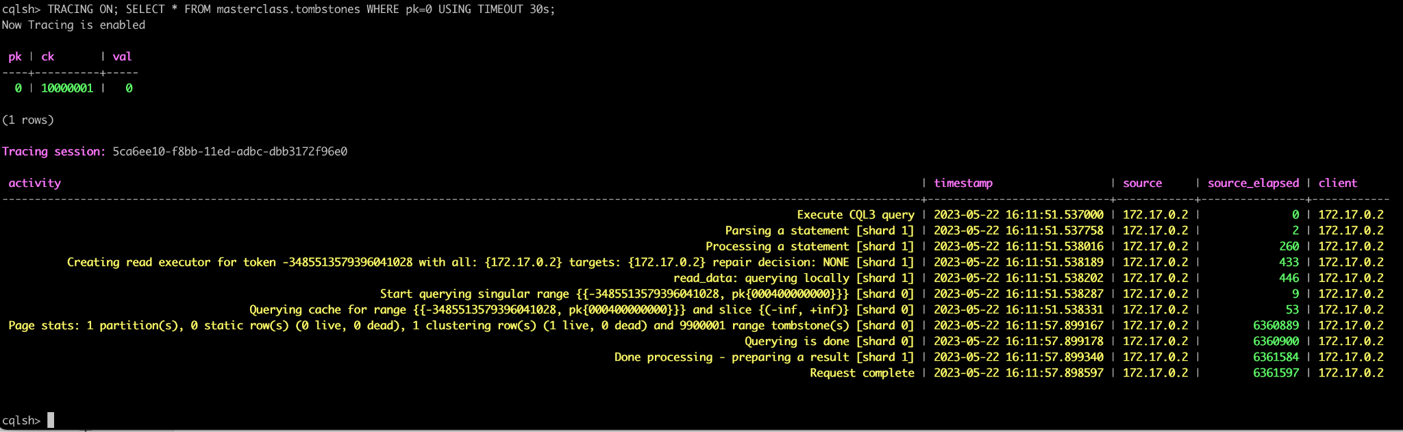
easy-cass-stress Joins the Apache Cassandra Project
I’m taking a quick break from my series on Cassandra node density to share some news with the Cassandra community: easy-cass-stress has officially been donated to the Apache Software Foundation and is now part of the Apache Cassandra project ecosystem as cassandra-easy-stress.
Why This Matters
Over the past decade, I’ve worked with countless teams struggling with Cassandra performance testing and benchmarking. The reality is that stress testing distributed systems requires tools that can accurately simulate real-world workloads. Many tools make this difficult by requiring the end user to learn complex configurations and nuance. While consulting at The Last Pickle, I set out to create an easy to use tool that lets people get up and running in just a few minutes