ScyllaDB X Cloud: An Inside Look with Avi Kivity (Part 1)
ScyllaDB’s co-founder/CTO on the motivations and architectural shifts behind ScyllaDB X Cloud — focusing on Raft and tablets-based data distribution If you follow ScyllaDB, you’ve probably heard us talking about Raft and tablets-based data distribution for a few years now. The ultimate goal of these projects (plus a few related ones) was to optimize elasticity and price performance – especially for dynamic and storage-bound workloads. And we finally hit a nice milestone along that journey: the release of ScyllaDB X Cloud. You can read about the release in our earlier blog post. Here, we wanted to share the engineering perspective on these architectural shifts. Tim Koopmans recently sat down with Avi Kivity – ScyllaDB Co-Founder and CTO – to chat about the underlying motivation and design decisions. You can watch the complete video here. But if you prefer to read, we’re writing up the highlights. This is the first blog post in a three-part series. Why ScyllaDB X Cloud? For scaling large clusters Tim: Let’s start with a big picture. What really motivated the architectural evolution behind what we know as ScyllaDB X Cloud? Was this change inevitable? How did it come into place? Avi: It came from our experience managing clusters for our customers. With the existing architecture, things like scaling up the cluster in preparation for events like Black Friday could take a long time. Since ScyllaDB can manage very large nodes (e.g., nodes with 30TB of data), moving that data onto new nodes could take a long time, sometimes a day. Also, nodes had to be added one at a time. If you had a large cluster, scaling the cluster would be a nail-biting experience. So we decided to improve that experience and, along the way, we improved many parts of the architecture. Tim: Do you have any numbers around what it used to be like to scale a large cluster? Avi: One of our large clusters has 75 nodes, each of which has around 60TB. It’s a pretty hefty cluster. It’s nice watching clusters like that on our dashboards and seeing compactions at tens of gigabytes per second aggregate across the cluster. Those clusters are churning through large amounts of data per second and carrying a huge amount of data. Now, we can scale this amount of data in minutes, maybe an hour for the most extreme cases. So it’s quite a huge change. Why ScyllaDB addressed scaling with Tablets & Raft Tim: When you think about dynamic or storage-bound workloads today, what are other databases getting wrong in this space? How did that lead you to this new approach, with tablets? Avi: “Other databases” is a huge area – there are hundreds of databases. Let’s talk about our heritage. We came from the Cassandra model. And the basic problem there was the static distribution of data. The node layout determines how data is distributed, and as long as you don’t add or remove nodes, it remains static. That means you have no flexibility. Also, the focus on having availability over consistency led to no central point for managing the topology. Without a coordinating authority, you could make only one change at a time. One of the first changes that we made was to add a coordinating authority in the form of Raft. Before, we managed topology with Gossip, which really puts cluster management responsibility on the operator. We moved it to a Raft group to centralize the management. You’ve probably heard the old proverb that anything in computer science can be solved with another layer of indirection. We did that with tablets, more or less. We inserted a layer of indirection so that instead of having a static distribution of data to nodes, it goes through a translation table. Each range of rows is mapped to a different node in a tablets table. By manipulating the tablets table, we can redirect small packages of data (specifically, 5GB – that’s pretty small for us). We can redirect the granularity of 5GB to any node and any CPU on any node. We can move those packages around at will, and those packages are moved at the line rate, so it’s no problem to fire them away at gigabits per second across the cluster. And that gives us the ability to rebalance data on a cluster or add and remove nodes very quickly. Tim: So tablets are really a new ScyllaDB abstraction? Is it an abstraction that breaks those tables into independently managed units? And I think you said the size is 5GB – is that configurable? Avi: It’s configurable, but I don’t recommend playing with it. Normally, you stay between 2.6GB and 10GB. When it reaches 10GB, it triggers a split, which will bring it back to 5GB. So each tablet will be split into two. If it goes down to 2.5GB, it will trigger a merge, merging two tablets into one larger tablet – again, bringing it back to 5GB. Tim: So ensuring that things can be dynamically split…We can move data around, rebalance across the cluster…That gives us finer-grained load distribution as well as better scalability and perhaps a bit of separation between compute and storage, right? Because we’re not necessarily tied to the size of the compute node anymore. We can have different instance types in a cluster now, as an indirect result of this change. The tipping point Tim: Avi, you said that re-architecting around tablets has been a huge shift. So what was the tipping point? Was it just that vNodes didn’t work anymore in terms of how you organize data? What was your aha moment where you said, “Yeah, I think we need to do something different here”? Avi: It was a combination of things, and since this was such a major change, we needed a lot of motivation to do it. One part of it was the inability to perform topology changes that involve more than one node at a time. Another part was that the previous streaming mechanism was very slow. Yet another part is that, because the streaming mechanism was so slow, we had to scale well in advance of exhausting the storage on the node. That required us to leave a lot of free space on the node, and that’s wasteful. We took all of this into consideration, and that was enough motivation for us to take on a multi-year change. I think it was well worth it. Tim: Multiyear…So how long ago did you start workshopping different ideas to solve? Avi: The first phase was changing topology to be strongly consistent and having a central authority to coordinate it. I think it took around a couple of years to switch to Raft topology. Before that, we switched schema management to use Raft as well. That was a separate problem, but since those two problems had the same solution, we jumped on it. We’re still not completely done. There are still a few features that are not yet fully compatible with tablets – but we see the light at the end of the tunnel now. [Stay tuned for parts 2 and 2]Be Part of Something Big – Speak at Monster Scale Summit
Share your “extreme scale engineering” expertise with ~20K like-minded engineers Whether you’re designing, implementing, or optimizing systems that are pushed to their limits, we’d love to hear about your most impressive achievements and lessons learned – at Monster Scale Summit 2026. Become a Monster Scale Summit Speaker What’s Monster Scale Summit? Monster Scale Summit is a technical conference that connects the community of people working on performance-sensitive data-intensive applications. Engineers, architects, and SREs from gamechangers around the globe will be gathering virtually to explore “monster scale” challenges with respect to extreme levels of throughput, data, and global distribution. It’s a lot like P99 CONF (also hosted by ScyllaDB) – a two-day event that’s free, fully virtual, and highly interactive. The core difference is that it’s focused on extreme scale engineering vs. all things performance. Last time, we hosted industry giants like Kelsey Hightower, Martin Kleppmann, Discord, Slack, Canva… Browse past sessions Details please! When: March 11 + 12 Where: Wherever you’d like! It’s intentionally virtual, so you can present and interact with attendees from anywhere around the world. Topics: Core topics include distributed databases, streaming and real-time processing, intriguing system designs, methods for balancing latency/concurrency/throughput, SRE techniques proven at scale, and infrastructure built for unprecedented demands. What we’re looking for: We welcome a broad range of talks about tackling the challenges that arise in the most massive, demanding environments. The conference prioritizes technical talks sharing first-hand experiences. Sessions are just 18-20 minutes – so consider this your TED Talk debut! Share your ideasBeyond Apache Cassandra
ScyllaDB is no longer “just” a faster Cassandra. In 2008, Apache Cassandra set a new standard for database scalability. Born to support Facebook’s Inbox Search, it has since been adopted by tech giants like Uber, Netflix, and Apple – where it’s run by experts who also serve as Cassandra contributors (alongside DataStax/IBM). And as its adoption scaled, Cassandra remained true to its core mission of scaling on commodity hardware with high availability. But what about performance? Simplicity? Efficiency? Elasticity? In 2015, ScyllaDB was born to go beyond Cassandra’s suboptimal resource utilization. Fresh from creating KVM and hacking the Linux kernel, the founders believed that their low-level engineering approach could squeeze considerably more power from the underlying infrastructure. The timing was ideal: just a year earlier, Netflix had published their numbers showing how to push Apache Cassandra to 1 million write RPS. This was an impressive feat, but one that required significant infrastructure investments and tuning efforts. The idea was quite simple (in theory, at least): take Apache Cassandra’s scalable architecture and reimplement it close to the metal while keeping wire protocol compatibility. Not relying on Java meant less latency variability (plus no stop the world pauses), while a unique shard-per-core architecture maximized servers’ throughput even under heavy system load. To prevent contention, everything was made asynchronous, and all these optimizations were paired with autonomous internal schedulers for minimal operational overhead. That was 10 years ago. While I can’t speak to Cassandra’s current direction, ScyllaDB evolved quite significantly since then – shifting from “just” a faster Cassandra alternative to a database with its own identity and unique feature set. Spoiler: In this video, I walk you through some key differences between ScyllaDB and how it differs from Apache Cassandra. I discuss the differences in performance, elasticity, and capabilities such as workload prioritization. You can see how ScyllaDB maps data per CPU core, scales in parallel, and de-risks topology changes—allowing it to handle millions of OPS with predictable low latencies (and without constant tuning and babysitting). ScyllaDB’s Evolution The first generation of ScyllaDB was all about raw performance. That’s when we introduced the shard-per-core asynchronous architecture, row-based cache, and advanced schedulers that achieve predictable low latencies. ScyllaDB’s second generation aimed for feature parity with Cassandra, but we actually went beyond that. For example, we introduced our Materialized views and production-ready Global Secondary Indexes (something that Cassandra still flags as experimental). Likewise, ScyllaDB also introduced support for local secondary indexes in that same year; those were just introduced in Cassandra 5 (after at least three different indexing implementations). Moreover, our Paxos implementation for lightweight transactions eliminated much of the overhead and limitations in Cassandra’s alternative implementation. The third generation marked our shift to the cloud, along with continued innovation. This is when ScyllaDB Alternator—our DynamoDB-compatible API—was introduced. We added support for ZSTD compression in 2020 (Cassandra only adopted it late in 2021). During this period, we dramatically improved repair speeds with row-level repair and introduced workload prioritization (more on this in the next section). The fourth generation of ScyllaDB emerged around the time AWS announced their i3en instance family, with high-density nodes holding up to 60TB of data (something Cassandra still struggles to handle effectively). During this period, we introduced the Incremental Compaction Strategy (ICS), allowing users to utilize up to 70% of their storage before scaling out. This later evolved into a hybrid compaction strategy (and we now support 90% storage utilization). We also introduced Change Data Capture (CDC) with a fundamentally different approach from Cassandra’s. And we significantly extended the CQL protocol with concepts such as shard-awareness, BYPASS CACHE, per-query configurable TIMEOUTs, and much more. Finally, we arrive at the fifth generation of ScyllaDB, which is still unfolding. This phase represents our path toward strong consistency and elasticity with Raft and Tablets. For more about the significance of this, read on… Capabilities That Set ScyllaDB Apart Our engineers have introduced lots of interesting features over the past decade. Based on my interactions with former Cassandra users, I think these are the most interesting to discuss here. Tablets Data Distribution Each ScyllaDB table is split into smaller fragments (“tablets”) to evenly distribute data and load across the system. Tablets bring elasticity to ScyllaDB, allowing you to instantly double, triple, or even 10x your cluster size to accommodate unpredictable traffic surges. They also enable more efficient use of storage, reaching up to 90% utilization. Since teams can quickly scale out in response to traffic spikes, they can satisfy latency SLAs without needing to overprovision “just in case.” Raft-based Strong Consistency for Metadata Raft introduces strong consistency to ScyllaDB’s metadata. Gone are the days when a schema change could push your cluster into disagreement or you’d lose access because you forgot to update the replication factor of your authentication keyspace (issues that still plague Cassandra). Workload Prioritization Workload prioritization allows you to consolidate multiple workloads under a single cluster, each with its own SLA. Basically, it controls how different workloads compete for system resources. Teams use it to prioritize urgent application requests that require immediate response times versus others that can tolerate slighter delays (e.g., large scans). Common use cases include balancing real-time vs batch processing, splitting writes from reads, and workload/infrastructure consolidation. Repair-based Operations Repair-based operations ensure your cluster data stays in sync, even during topology changes. This addresses a long-standing data consistency flaw in Apache Cassandra, where operations like replacing failed nodes can result in data loss. ScyllaDB also fully eliminates the problem of data resurrection, thanks to repair-based tombstone garbage collection. Incremental Compaction Incremental compaction (ICS) has been the default compaction strategy in ScyllaDB for over five years. ICS greatly reduces the temporary space amplification, resulting in more disk space being available for storing user data – and that eliminates the typical requirement of 50% free space in your drive. There is no comparable Cassandra feature. Cassandra just recently introduced Unified Compaction, which has yet to prove itself. Row-based Cache ScyllaDB’s row-based cache is also unique. It is enabled by default and requires no manual tuning. With the BYPASS CACHE extension, you can prevent cache pollution by keeping important items from being invalidated. Additionally, SSTable index caching significantly reduces I/O access time when fetching data from disk. Per-shard Concurrency Limits and Rate Limiters ScyllaDB includes per-shard concurrency limits and rate limiters per partition to protect against unexpected spikes. Whether dealing with a misbehaving client or a flood of requests to a specific key, ScyllaDB ensures resilience where Cassandra often falls short. DynamoDB Compatibility ScyllaDB also offers a DynamoDB-compatible layer, further distancing itself from its Apache Cassandra origins. This lets teams run their DynamoDB workloads on any cloud or on-prem – without code changes, and with 50% lower cost. This has helped quite a few teams consolidate multiple workloads on ScyllaDB. What’s Next? At the recent Monster SCALE Summit, CEO/co-founder Dor Laor shared a peek at what’s next for ScyllaDB. A few highlights… Ready now (see this blog post and product page for details): The ability to safely run at 90% storage utilization Support for clusters with mixed instance type nodes Dynamic provisioning and flex credit Short-term: Vector search Strongly consistent tables Fault injection service Transparent repairs Object and tiered storage Raft for strongly consistent tables Longer-term Multi-key transactions Analytics and transformations with UDFs Automated large partition balancing Immutable infrastructure for greater stability and reliability A replication mode for more flexible and efficient infrastructure changes For details, watch the complete talk here: To close, ScyllaDB is faster than Cassandra (I’ll share our latest benchmark results here soon). But both ScyllaDB and Cassandra have evolved to the point that ScyllaDB is no longer “just” a faster Cassandra. We’ve evolved beyond Cassandra. If your project needs more predictable performance – and/or could benefit from the elasticity, efficiency, and simplicity optimizations we’ve been focusing on for years now – you might also want to consider evolving beyond Cassandra.We Built a Tool to Diagnose ScyllaDB Kubernetes Issues
Introducing Scylla Operator Analyze, a tool to help platform engineers and administrators deploy ScyllaDB clusters running on Kubernetes Imagine it’s a Friday afternoon. Your company is migrating all the data to ScyllaDB and you’re in the middle of setting up the cluster on Kubernetes. Then, something goes wrong. Your time today is limited, but the sheer volume of ScyllaDB configuration feels endless. To help you detect problems in ScyllaDB deployments, we built Scylla Operator Analyze, a command-line tool designed to automatically analyze Kubernetes-based ScyllaDB clusters, identify potential misconfigurations, and offer actionable diagnostics. In modern infrastructure management, Kubernetes has revolutionized how we orchestrate containers and manage distributed systems. However, debugging complex Kubernetes deployments remains a significant challenge, especially in production-grade, high-performance environments like those powered by ScyllaDB. In this blog post, we’ll explain what Scylla Operator Analyze is, how it works, and how it may help platform engineers and administrators deploy ScyllaDB clusters running on Kubernetes. The repo we’ve been working on is available here. It’s a fork of Scylla Operator, but the project hasn’t been merged upstream (it’s highly experimental). What is Scylla Operator Analyze? Scylla Operator Analyze is a Go-based command-line utility that extends Scylla Operator by introducing a diagnostic command. Its goal is straightforward: automatically inspect a given Kubernetes deployment and report problems it identified in the deployment configuration. We designed our tool to help ScyllaDB’s technical support staff to quickly diagnose known issues reported by our clients, both by providing solutions for simple problems, and helpful insights in more complex cases. However, it’s also freely available as a subcommand of the Scylla Operator binary. The next few sections share how we implemented the tool. If you want to go straight to example usage, skip to the Making a diagnosis section. Capturing the cluster state Kubernetes deployments consist of many components with various functions. Collectively, they are called resources. The Kubernetes API presents them to the client as objects containing fields with information about their configuration and current state. Two modes of operation Scylla Operator Analyze supports two ways of collecting these data: Live Cluster Connection The tool can connect directly to a Kubernetes cluster using the client-go API. Once connected, it retrieves data from Kubernetes resources and compiles it into an internal representation. Archive-Based Analysis (Must-Gather) Alternatively, the tool can analyze archived cluster states created using a utility calledmust-gather. These archives
contain YAML descriptions of resources, allowing offline analysis.
Diagnosis by analyzing symptoms Symptoms are high-level objects
representing certain issues that could occur while deploying a
ScyllaDB cluster. A symptom contains the diagnosis of the problem
and a suggestion on how to fix it, as well as a method for checking
if the problem occurs in a given deployment (we cover this in the
section about selectors). In order to create objects representing
more complex problems, symptoms can be used to create tree-like
structures. For example, a problem that could manifest itself in a
few different ways could be represented by many symptoms checking
for all the different spots the problem could affect. Those
symptoms would be connected to one root symptom, describing the
cause of the problem. This way, if any of the sub-symptoms report
that their condition is met, the tool can display the root cause
instead of one specific manifestation of that problem. Example
of a symptom and the workflow used to detect it. In this
example, let’s assume that the driver is unable to provide storage,
but NodeConfig does not report a nonexistent device. When checking
if the symptom occurs, the tool will perform the following steps.
Check if the NodeConfig reports a nonexistent device – no Check if
the driver is unable to provide storage – yes. At this point we
know the symptom occurs, so we don’t need to check for any more
subsymptoms. Since one of the subsymptoms occurs, the main symptom
(NodeConfig configured with nonexistent volume) is reported to the
user. Deployment condition description Resources As described
earlier, Kubernetes deployments can be considered collections of
many interconnected resources. All resources are described using
so-called fields. Fields contain information identifying resources,
deployment configuration and descriptions of past and current
states. Together, these data give the controllers all the
information they need to supervise the deployment. Because of that,
they are very useful for debugging issues and are the main source
of information for our tool. Resources’ fields contain a special
kind field, which describes what the resource is and
indicates what other fields are available. Some fundamental
Kubernetes resource kinds include Pods, Services, etc. Those can
also be extended with custom ones, such as the
ScyllaCluster resource kind defined by the Scylla
Operator. This provides the most basic kind of grouping of
resources in Kubernetes. Other fields are grouped in sections
called Metadata, which provide identifying information,
Spec, which contain configuration and Status,
which contain current status. Such a description in YAML format may
look something like this: apiVersion: v1 kind: Pod metadata:
creationTimestamp: "2024-12-03T17:47:06Z" labels: scylla/cluster:
scylla scylla/datacenter: us-east-1 scylla/scylla-version: 6.2.0
name: scylla-us-east-1-us-east-1a-0 namespace: scylla spec:
volumes: - name: data persistentVolumeClaim: claimName:
data-scylla-us-east-1-us-east-1a-0 status: conditions: -
lastTransitionTime: "2024-12-03T17:47:06Z" message: '0/1 nodes are
available: pod has unbound immediate PersistentVolumeClaims.
preemption: 0/1 nodes are available: 1 Preemption is not helpful
for scheduling.' reason: Unschedulable status: "False" type:
PodScheduled phase: Pending Selectors An accurate
description of symptoms (presented in the previous section)
requires a method for describing conditions in the deployment using
information contained in the resources’ fields. Moreover, because
of the distributed nature of both Kubernetes deployments and
ScyllaDB, these descriptions must also specify how the resources
are related to one another. Our tool comes with a package providing
selectors. They offer a simple, yet powerful, way to
describe deployment conditions using Kubernetes objects in a way
that’s flexible and allows for automatic processing using the
provided selection engine. A selector can be thought of as a query
because it specifies the kinds of resources to select and criteria
which they should satisfy. Selectors are constructed using four
main methods of the selector structure builder. First, the
developer specifies resources to be selected with the
Select method by specifying their kind and a predicate
which should be true for the selected resources. The predicate is
provided as a standard Go closure to allow for complex conditions
if needed. Next, the developer may call the Relate method
to define a relationship between two kinds of resources. This is
again defined using a Go closure as a predicate, which must hold
for the two objects to be considered in the same result set. This
can establish a context within which an issue should be inspected
(for example: connecting a Pod to relevant Storage resources).
Finally, constraints for individual resources in the result set can
be specified with the Where method, similarly to how it is
done in the Select method. This method is mainly meant to
be used with the SelectWithNil method. The
SelectWithNil method is the same as the Select
method; the only difference is that it allows returning a special
nil value instead of a resource instance. This
nil value signifies that no resources of a given
kind match all the other resources in the resulting set. Thanks to
this, selectors can also be used to detect a scenario where a
resource is missing just by examining the context of related
resources. An example selector — shortened for brevity — may look
something like this: selector. New(). Select("scylla-pod",
selector.Type[*v1.Pod](), func(p *v1.Pod) (bool, error) { /* ... */
}). SelectWithNil("storage-class",
selector.Type[*storagev1.StorageClass](), nil). Select("pod-pvc",
selector.Type[*v1.PersistentVolumeClaim](), nil).
Relate("scylla-pod", "pod-pvc", func(p *v1.Pod, pvc
*v1.PersistentVolumeClaim) (bool, error) { for _, volume := range
p.Spec.Volumes { vPvc := volume.PersistentVolumeClaim if vPvc !=
nil && (*vPvc).ClaimName == pvc.Name { return true, nil } }
return false, nil }). Relate("pod-pvc", "storage-class", /* ...
*/). Where("storage-class", func(sc *storagev1.StorageClass) (bool,
error) { return sc == nil, nil }) In symptom definitions,
selectors for a corresponding condition are used and are usually
constructed alongside them. Such a selector provides a description
of a faulty condition. This means that if there is a matching set
of resources, it can be inferred that the symptom occurs. Finally,
the selector can then be used, given all the deployments resources,
to construct an iterator-like object that provides a list of all
the sets of resources that match the selector. Symptoms can then
use those results to detect issues and generate diagnoses
containing useful debugging information. Making a diagnosis When a
symptom relating to a problematic condition is detected, a
diagnosis for a user is generated. Diagnoses are
automatically generated report objects summarizing the problem and
providing additional information. A diagnosis consists of
an issue description, identifiers of resources related to the
fault, and hints for the user (when available). Hints may contain,
for example, a description of steps to remedy the issue or a
reference to a bug tracker. In the final stage of analysis, those
diagnoses are presented to the user and the output may look
something like this: Diagnoses: scylladb-local-xfs StorageClass
used by a ScyllaCluster is missing Suggestions: deploy
scylladb-local-xfs StorageClass (or change StorageClass) Resources
GVK: /v1.PersistentVolumeClaim,
scylla/data-scylla-us-east-1-us-east-1a-0 (4…)
scylla.scylladb.com/v1.ScyllaCluster, scylla/scylla
(b6343b79-4887-497b…) /v1.Pod, scylla/scylla-us-east-1-us-east-1a-0
(0e716c3f-6432-4eeb-b5ff-…) Learn more As we suggested, Kubernetes
deployments of ScyllaDB involve many interacting components, each
of which has its own quirks. Here are a few strategies to help in
diagnosing the problems you encounter: Run
Scylla Doctor Check our troubleshooting
guide Look for open
issues on our GitHub Check our forum Ask us on Slack Learn more about
ScyllaDB at ScyllaDB
University Good luck, fellow troubleshooter! Building easy-cass-mcp: An MCP Server for Cassandra Operations
I’ve started working on a new project that I’d like to share, easy-cass-mcp, an MCP (Model Context Protocol) server specifically designed to assist Apache Cassandra operators.
After spending over a decade optimizing Cassandra clusters in production environments, I’ve seen teams consistently struggle with how to interpret system metrics, configuration settings, schema design, and system configuration, and most importantly, how to understand how they all impact each other. While many teams have solid monitoring through JMX-based collectors, extracting and contextualizing specific operational metrics for troubleshooting or optimization can still be cumbersome. The good news is that we now have the infrastructure to make all this operational knowledge accessible through conversational AI.
How GE Healthcare Took DynamoDB on Prem for Its AI Platform
How GE Healthcare moved a DynamoDB‑powered AI platform to hospital data centers, without rewriting the app How do you move a DynamoDB‑powered AI platform from AWS to hospital data centers without rewriting the app? That’s the challenge that Sandeep Lakshmipathy (Director of Engineering at GE Healthcare) decided to share with the ScyllaDB community a few years back. We noticed an uptick in people viewing this video recently, so we thought we’d share it here, in blog form. Watch or read, your choice. Intro Hi, I’m Sandeep Lakshmipathy, the Director of Engineering for the Edison AI group at GE Healthcare. I have about 20 years of experience in the software industry, working predominantly in product and platform development. For the last seven years I’ve been in the healthcare domain at GE, rolling out solutions for our products. Let me start by setting some context with respect to the healthcare challenges that we face today. Roughly 130M babies are born every year; about 350K every single day. There’s a 40% shortage of healthcare workers to help bring these babies into the world. Ultrasound scans help ensure the babies are healthy, but those scans are user‑dependent, repetitive, and manual. Plus, clinical training is often neglected. Why am I talking about this? Because AI solutions can really help in this specific use case and make a big difference. Now, consider this matrix of opportunities that AI presents. Every single tiny dot within each cell is an opportunity in itself. The newborn‑baby challenge I just highlighted is one tiny speck in this giant matrix. It shows what an infinite space this is, and how AI can address each challenge in a unique way. GE Healthcare is tackling these opportunities through a platform approach. Edison AI Workbench (cloud) We ingest data from many devices and customers: scanners, research networks, and more. Data is then annotated and used to train models. Once the models are trained, we deploy them onto devices. The Edison AI Workbench helps data scientists view and annotate data, train models, and package them for deployment. The whole Edison AI Workbench runs in AWS and uses AWS resources to provide a seamless experience to the data scientists and annotators who are building AI solutions for our customers. Bringing Edison AI Workbench on‑prem When we showed this solution to our research customers, they said, “Great, we really like the features and the tools….but can we have Edison AI Workbench on‑prem?” So, we started thinking: How do we take something that lives in the AWS cloud, uses all those resources, and relies heavily on AWS services – and move it onto an on‑prem server while still giving our research customers the same experience? That’s when we began exploring different options. Since DynamoDB was one of the main things tying us to the AWS cloud, we started looking for a way to replace it in the on‑prem world. After some research, we saw that ScyllaDB was a good DynamoDB replacement because it provides API compatibility with DynamoDB. Without changing much code and keeping all our interfaces the same, we migrated the Workbench to on‑prem and quickly delivered what our research customers asked for. Why ScyllaDB Alternator (DynmamoDB-Compatible API)? Moving cloud assets on‑prem is not trivial; expertise, time‑to‑market, service parity, and scalability all matter. We also wanted to keep our release cycles short: in the cloud we can push features every sprint; on‑prem, we still need regular updates. Keeping the database layer similar across cloud and on‑prem minimized rework. Quick proofs of concept confirmed that ScyllaDB + Alternator met our needs, and using Kubernetes on‑prem let us port microservices comfortably. The ScyllaDB team has always been available with respect to developer‑level interactions, quick fixes in nightly builds, and constant touch‑points with technical and marketing teams. All of this helped us move fast. For example, DynamoDB Streams wasn’t yet in ScyllaDB when we adopted it (back in 2020), but the team provided work‑arounds until the feature became available. They also worked with us on licensing to match our needs. This partnership was crucial to the solution’s evolution. By partnering with the ScyllaDB team, we could take a cloud‑native Workbench to our on‑prem research customers in healthcare. Final thoughts Any AI solution rollout depends on having the right data volume and balance. It’s all the annotations that drive model quality. Otherwise, the model will be brittle, and it won’t have the necessary diversity. Supporting all these on‑prem Workbench use cases helps because it takes the tools to where the data is. The cloud workbench handles data in the cloud data lake. But at the same time, our research customers who are partnering with us can use this on-prem, taking the tools to where the data is: in their hospital network.Real-Time Database Read Heavy Workloads: Considerations and Best Practices
Explore the challenges associated with real-time read-heavy database workloads and get tips for addressing them Reading and writing are distinctly different beasts. This is true with reading/writing words, reading/writing code, and also when we’re talking about reading/writing data to a database. So, when it comes to optimizing database performance, your read:write ratio really does matter. We recently wrote about performance considerations that are important for write-heavy workloads – covering factors like LSM tree vs B-tree engines, payload size, compression, compaction, and batching. But read-heavy database workloads bring a different set of challenges; for example: Scaling a cache: Many teams try to speed up reads by adding a cache in front of their database, but the cost and complexity can become prohibitive as the workload grows. Competing workloads: Things might work well initially, but as new use cases are added, a single workload can end up bottlenecking all the others. Constant change: As your dataset grows or user behaviors shift, hotspots might surface. In this article, we explore high-level considerations to keep in mind when you have a latency-sensitive read-heavy workload. Then, we’ll introduce a few ScyllaDB capabilities and best practices that are particularly helpful for read-heavy workloads. What Do We Mean by “a Real-Time Read Heavy Workload”? First, let’s clarify what we mean by a “real-time read-heavy” workload. We’re talking about workloads that: Involve a large amount of sustained traffic (e.g., over 50K OPS) Involve more reads than writes Are bound by strict latency SLAs (e.g., single digit millisecond P99 latency) Here are a few examples of how they manifest themselves in the wild: Betting: Everyone betting on a given event is constantly checking individual player, team, and game stats as the match progresses. Social networks: A small subset of people are actually posting new content, while the vast majority of users are typically just browsing through their feeds and timelines. Product Catalogs: As with social media, there’s a lot more browsing than actual updating. Considerations Next, let’s look at key considerations that impact read performance in real-time database systems. The Database’s Read Path To understand how databases like ScyllaDB process read operations, let’s recap its read path. When you submit a read (a SELECT statement), the database first checks for the requested data in memtables, which are in-memory data structures that temporarily hold your recent writes. Additionally, the database checks whether the data is present in the cache. Why is this extra step necessary? Because the memtable may not always hold the latest data. Sometimes data could be written out-of-order, especially if applications consume data from unordered sources. As the protocol allows for clients to manipulate record timestamps to prevent correct ordering, checking both the memtable and the cache is necessary to ensure that the latest write takes gets returned. Then, the database takes one of two actions: If the data is stored on the disk, the database populates the cache to speed up subsequent reads. If the data doesn’t exist on disk, the database notes this absence in the cache – avoiding further unnecessary lookups there. As memtables flush to disk, the data also gets merged with the cache. That way, the cache ends up reflecting the latest on-disk data. Hot vs. Cold Reads Reading from cache is always faster than reading from disk. The more data your database can serve directly from cache, the better its performance (since reading data from memory has a practically unlimited fetch ceiling). But how can you tell whether your reads are going to cache or disk? Monitoring. You can use tools such as the ScyllaDB Monitoring stack to learn all about your cache hits and misses. The fewer cache misses, the better your read latencies. ScyllaDB uses a Least Recently Used (LRU) caching strategy, similar to Redis and Memcached. When the cache gets full, the least-accessed data is evicted to make room for new entries. With this LRU approach, you need to be mindful about your reads. You want to avoid situations where a few “expensive” reads end up evicting important items from your cache. If you don’t optimize cache usage, you might encounter a phenomenon called “cache thrashing.” That’s what happens when you’re continuously evicting and replacing items in your cache, essentially rendering the cache ineffective. For instance, full table scans can create significant cache pressure, particularly when your working set size is larger than your available caching space. During a scan, if a competing workload relies on reading frequently cached data, its read latency will momentarily increase because those items were evicted. To prevent this situation, expensive reads should specify options like ScyllaDB’s BYPASS_CACHE to prevent its results from evicting important items. Paging Paging is another important factor to consider. It’s designed to prevent the database from running out of memory when scanning through large results. Basically, rows get split into pages as defined by your page size, and selecting an appropriate page size is essential for minimizing end-to-end latency. For example, assume you have a quorum read request in a 3-node cluster. Two replicas must respond for the request to be successful. Each replica computes a single page, which then gets reconciled by the coordinator before returning data back to the client. Note that: ScyllaDB latencies are reported per page. If your application latencies are high, but low on the database side, it is an indication that your clients may be often paging. Smaller page sizes increase the number of client-server roundtrips. For example, retrieving 1,000 rows with a page size of 10 requires 100 client-server round trips, impacting latency. Testing various page sizes helps finding the optimal balance. Most drivers default to 5,000 rows per page, which works well in most cases, but you may want to increase from the defaults when scanning through wide rows, or during full scans – at the expense of letting the database work more before receiving a response. Sometimes trial and error is needed to get the page size nicely tuned for your application. Tombstones In Log-Structured Merge-tree (LSM-tree) databases like ScyllaDB, handling tombstones (markers for deleted data) is also important for read performance. Tombstones ensure that deletions are properly propagated across replicas to avoid deleted data from being “resurrected.” They’re critical for maintaining correctness. However, read-heavy workloads with frequent deletions may have to process lots of tombstones to return a single page of live data. This can really impact latency. For example, consider this extreme example. Here, tracing data shows that a simple select query took a whopping 6 seconds to process a single row because it had to go through 10 million tombstones. There are a couple ways to avoid this: tuning compaction strategies, such as the more aggressive LeveledCompactionStrategy, or using ICS Space Amplification Goal, or optimizing your access patterns to scanning through fewer dead rows on every point query. Optimizing Read-Heavy Workloads with ScyllaDB While ScyllaDB’s LSM tree storage engine makes it quite well-suited for write-heavy workloads, our engineers have introduced a variety of features that optimize it for ultra-low latency reads as well. ScyllaDB Cache One of ScyllaDB’s key components for achieving low latency is its unique caching mechanism. Many databases rely on the operating system’s page cache, which can be inefficient and doesn’t provide the level of control needed for predictable low latency. The OS cache lacks workload-specific context, making it difficult to prioritize which items should remain in memory and which can be safely evicted. At ScyllaDB, our engineering team addressed this by implementing our own unified internal cache. When ScyllaDB starts, it locks most of the server’s memory and directly manages it, bypassing the OS cache. Additionally, ScyllaDB’s cache uses a shared-nothing approach, giving each shard/vCPU its own cache, memtable, and SSTable. This eliminates the need for concurrency locks and reduces context switching, further maximizing performance. You can read more about that unified cache in this engineering blog post. SSTable Index Caching Another performance-focused feature of ScyllaDB is its ability to cache SSTable indexes in memory. Since working sets often exceed the memory available, reads sometimes go to disk. However, disk access is costly. By caching SSTable indexes, ScyllaDB reduces disk IO costs by up to 3x. This significantly improves read performance – particularly during cache misses. ScyllaDB’s index caching is demand-driven: entries are cached upon access and evicted on demand. If your workload reads heavily from disk, it’s often helpful to increase the size of this index cache. Workload Prioritization Competing workloads can lead to latency issues, as we mentioned at the beginning of this article. ScyllaDB provides a solution for this: its Workload Prioritization feature, which allows you to assign priority levels to different workloads. This is particularly useful if you have workloads with varying latency requirements, as it lets you prioritize latency-sensitive queries over others. You assign service levels to each workload, then ScyllaDB’s internal scheduler handles query prioritization according to those predefined levels. To learn more, see my recent talk from ScyllaDB Summit. Heat-Weighted Load Balancing (HWLB) Heat-Weighted Load Balancing (HWLB) is a powerful ScyllaDB feature that’s commonly overlooked. HWLB mitigates performance issues that can arise when a replica node restarts with a cold cache, like after a rolling restart for a configuration change or an upgrade. In such cases, other nodes notice that the replica’s cache is cold and gradually start directing requests to the restarted node until its cache eventually warms up. The HWLB algorithm controls how requests are routed to a cold replica. The mathematical formula behind this gradual allocation is shown above – it explains the pacing of requests sent to a node as it warms up. HWLB ensures that nodes with a cold cache do not immediately receive full traffic, in turn preventing abrupt latency spikes. When restarting ScyllaDB replicas, pay attention to the Reciprocal Miss Rate (HWLB) panel within the ScyllaDB Monitoring. Nodes with a higher ratio will serve more reads compared to other nodes. Prepared statements with ScyllaDB’s shard-aware drivers On the client side, using prepared statements is a critical best practice. A prepared statement is a query parsed by ScyllaDB and then saved for later use. Prepared statements allow ScyllaDB to route queries directly to replica nodes and shards that hold the requested data. Without prepared statements, a query may be routed to a node without the required data – resulting in extra round trips. With prepared statements, queries are always routed efficiently, minimizing network overhead and improving response times. Try it out: This ScyllaDB University lesson walks you through prepared statements. High concurrency Perhaps the most important tip here is to remember that ScyllaDB loves concurrency… but only up to a certain point. If you send too few requests to the database, you won’t be able to fully maximize its potential. However, if you have unbounded concurrency – you send too many requests to the database – that excessive concurrency can cause performance degradation. To find the sweet spot, apply this formula: *Concurrency = Throughput × Latency*. For example, if you want to run 200K operations per second with an average latency of 1ms, you would aim for a concurrency level of 200. Using this calculation, adjust your driver settings – setting the number of connections and maximum in-flight requests per connection to meet your target concurrency. If your driver settings yield a concurrency higher than needed, reduce them. If it’s lower, increase them accordingly. Wrapping Up As we’ve discussed, there are a lot of ways you can keep latencies low with read-heavy workloads – even on databases such as ScyllaDB which are also optimized for write-heavy workloads. In fact, ScyllaDB performance is comparable to dedicated caching solutions like Memcached for certain workloads. If you want to learn more, here are some firsthand perspectives from teams who tackled some interesting read-heavy challenges: Discord: With millions of users actively reading and searching chat history, Discord needs ultra-low-latency reads and high throughput to maintain real-time interactions at scale. Epic Games: To support Unreal Engine Cloud, Epic Games needed a high-speed, scalable metadata store that could handle rapid cache invalidation and support metadata storage for game assets. Zeroflucs: To power their sports betting application, ZeroFlucs had to process requests in near real-time, constantly, and in a region local to both the customer and the data. Also, take a look at the following video, where we go into even greater depth on these read-heavy challenges and also walk you through what these workloads look like on ScyllaDB.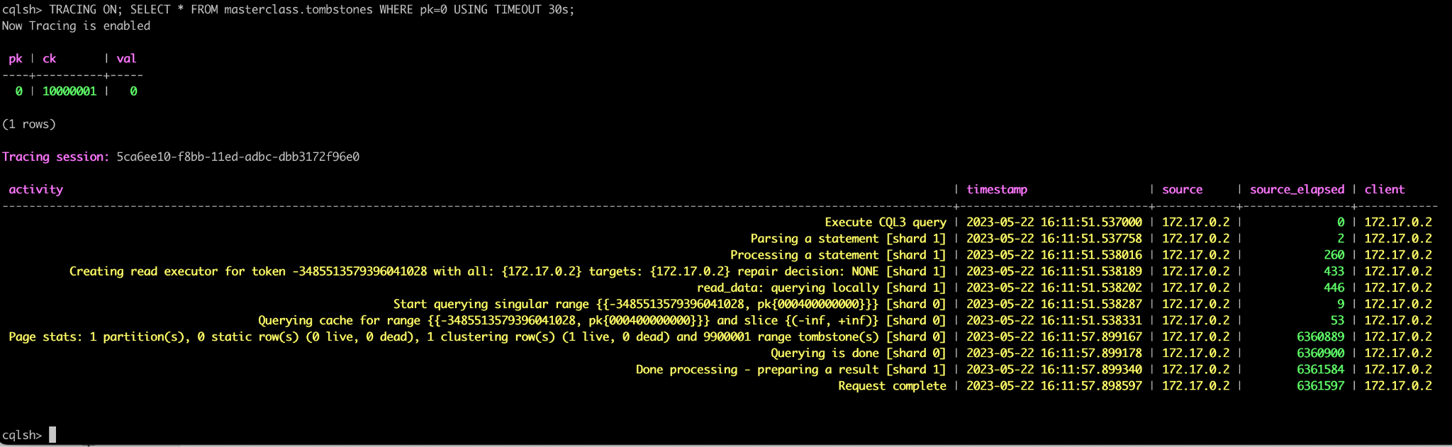
easy-cass-stress Joins the Apache Cassandra Project
I’m taking a quick break from my series on Cassandra node density to share some news with the Cassandra community: easy-cass-stress has officially been donated to the Apache Software Foundation and is now part of the Apache Cassandra project ecosystem as cassandra-easy-stress.
Why This Matters
Over the past decade, I’ve worked with countless teams struggling with Cassandra performance testing and benchmarking. The reality is that stress testing distributed systems requires tools that can accurately simulate real-world workloads. Many tools make this difficult by requiring the end user to learn complex configurations and nuance. While consulting at The Last Pickle, I set out to create an easy to use tool that lets people get up and running in just a few minutes
Azure fault domains vs availability zones: Achieving zero downtime migrations
The challenges of operating production-ready enterprise systems in the cloud are ensuring applications remain up to date, secure and benefit from the latest features. This can include operating system or application version upgrades, but it is not limited to advancements in cloud provider offerings or the retirement of older ones. Recently, NetApp Instaclustr undertook a migration activity for (almost) all our Azure fault domain customers to availability zones and Basic SKU IP addresses.
Understanding Azure fault domains vs availability zones
“Azure fault domain vs availability zone” reflects a critical distinction in ensuring high availability and fault tolerance. Fault domains offer physical separation within a data center, while availability zones expand on this by distributing workloads across data centers within a region. This enhances resiliency against failures, making availability zones a clear step forward.
The need for migrating from fault domains to availability zones
NetApp Instaclustr has supported Azure as a cloud provider for our Managed open source offerings since 2016. Originally this offering was distributed across fault domains to ensure high availability using “Basic SKU public IP Addresses”, but this solution had some drawbacks when performing particular types of maintenance. Once released by Azure in several regions we extended our Azure support to availability zones which have a number of benefits including more explicit placement of additional resources, and we leveraged “Standard SKU Public IP’s” as part of this deployment.
When we introduced availability zones, we encouraged customers to provision new workloads in them. We also supported migrating workloads to availability zones, but we had not pushed existing deployments to do the migration. This was initially due to the reduced number of regions that supported availability zones.
In early 2024, we were notified that Azure would be retiring support for Basic SKU public IP addresses in September 2025. Notably, no new Basic SKU public IPs would be created after March 1, 2025. For us and our customers, this had the potential to impact cluster availability and stability – as we would be unable to add nodes, and some replacement operations would fail.
Very quickly we identified that we needed to migrate all customer deployments from Basic SKU to Standard SKU public IPs. Unfortunately, this operation involves node-level downtime as we needed to stop each individual virtual machine, detach the IP address, upgrade the IP address to the new SKU, and then reattach and start the instance. For customers who are operating their applications in line with our recommendations, node-level downtime does not have an impact on overall application availability, however it can increase strain on the remaining nodes.
Given that we needed to perform this potentially disruptive maintenance by a specific date, we decided to evaluate the migration of existing customers to Azure availability zones.
Key migration consideration for Cassandra clusters
As with any migration, we were looking at performing this with zero application downtime, minimal additional infrastructure costs, and as safe as possible. For some customers, we also needed to ensure that we do not change the contact IP addresses of the deployment, as this may require application updates from their side. We quickly worked out several ways to achieve this migration, each with its own set of pros and cons.
For our Cassandra customers, our go to method for changing cluster topology is through a data center migration. This is our zero-downtime migration method that we have completed hundreds of times, and have vast experience in executing. The benefit here is that we can be extremely confident of application uptime through the entire operation and be confident in the ability to pause and reverse the migration if issues are encountered. The major drawback to a data center migration is the increased infrastructure cost during the migration period – as you effectively need to have both your source and destination data centers running simultaneously throughout the operation. The other item of note, is that you will need to update your cluster contact points to the new data center.
For clusters running other applications, or customers who are more cost conscious, we evaluated doing a “node by node” migration from Basic SKU IP addresses in fault domains, to Standard SKU IP addresses in availability zones. This does not have any short-term increased infrastructure cost, however the upgrade from Basic SKU public IP to Standard SKU is irreversible, and different types of public IPs cannot coexist within the same fault domain. Additionally, this method comes with reduced rollback abilities. Therefore, we needed to devise a plan to minimize risks for our customers and ensure a seamless migration.
Developing a zero-downtime node-by-node migration strategy
To achieve a zero-downtime “node by node” migration, we explored several options, one of which involved building tooling to migrate the instances in the cloud provider but preserve all existing configurations. The tooling automates the migration process as follows:
- Begin with stopping the first VM in the cluster. For cluster availability, ensure that only 1 VM is stopped at any time.
- Create an OS disk snapshot and verify its success, then do the same for data disks
- Ensure all snapshots are created and generate new disks from snapshots
- Create a new network interface card (NIC) and confirm its status is green
- Create a new VM and attach the disks, confirming that the new VM is up and running
- Update the private IP address and verify the change
- The public IP SKU will then be upgraded, making sure this operation is successful
- The public IP will then be reattached to the VM
- Start the VM
Even though the disks are created from snapshots of the original disks, we encountered several discrepancies in our testing, with settings between the original VM and the new VM. For instance, certain configurations, such as caching policies, did not automatically carry over, requiring manual adjustments to align with our managed standards.
Recognizing these challenges, we decided to extend our existing node replacement mechanism to streamline our migration process. This is done so that a new instance is provisioned with a new OS disk with the same IP and application data. The new node is configured by the Instaclustr Managed Platform to be the same as the original node.
The next challenge: our existing solution is built so that the replaced node was provisioned to be the exact same as the original. However, for this operation we needed the new node to be placed in an availability zone instead of the same fault domain. This required us to extend the replacement operation so that when we triggered the replacement, the new node was placed in the desired availability zone. Once this operation completed, we had a replacement tool that ensured that the new instance was correctly provisioned in the availability zone, with a Standard SKU, and without data loss.
Now that we had two very viable options, we went back to our existing Azure customers to outline the problem space, and the operations that needed to be completed. We worked with all impacted customers on the best migration path for their specific use case or application and worked out the best time to complete the migration. Where possible, we first performed the migration on any test or QA environments before moving onto production environments.
Collaborative customer migration success
Some of our Cassandra customers opted to perform the migration using our data center migration path, however most customers opted for the node-by-node method. We successfully migrated the existing Azure fault domain clusters over to the Availability Zone that we were targeting, with only a very small number of clusters remaining. These clusters are operating in Azure regions which do not yet support availability zones, but we were able to successfully upgrade their public IP from Basic SKUs that are set for retirement to Standard SKUs.
No matter what provider you use, the pace of development in cloud computing can require significant effort to support ongoing maintenance and feature adoption to take advantage of new opportunities. For business-critical applications, being able to migrate to new infrastructure and leverage these opportunities while understanding the limitations and impact they have on other services is essential.
NetApp Instaclustr has a depth of experience in supporting business critical applications in the cloud. You can read more about another large-scale migration we completed The worlds Largest Apache Kafka and Apache Cassandra Migration or head over to our console for a free trial of the Instaclustr Managed Platform.
The post Azure fault domains vs availability zones: Achieving zero downtime migrations appeared first on Instaclustr.
Integrating support for AWS PrivateLink with Apache Cassandra® on the NetApp Instaclustr Managed Platform
Discover how NetApp Instaclustr leverages AWS PrivateLink for secure and seamless connectivity with Apache Cassandra®. This post explores the technical implementation, challenges faced, and the innovative solutions we developed to provide a robust, scalable platform for your data needs.
Last year, NetApp achieved a significant milestone by fully integrating AWS PrivateLink support for Apache Cassandra® into the NetApp Instaclustr Managed Platform. Read our AWS PrivateLink support for Apache Cassandra General Availability announcement here. Our Product Engineering team made remarkable progress in incorporating this feature into various NetApp Instaclustr application offerings. NetApp now offers AWS PrivateLink support as an Enterprise Feature add-on for the Instaclustr Managed Platform for Cassandra, Kafka®, OpenSearch®, Cadence®, and Valkey™.
The journey to support AWS PrivateLink for Cassandra involved considerable engineering effort and numerous development cycles to create a solution tailored to the unique interaction between the Cassandra application and its client driver. After extensive development and testing, our product engineering team successfully implemented an enterprise ready solution. Read on for detailed insights into the technical implementation of our solution.
What is AWS PrivateLink?
PrivateLink is a networking solution from AWS that provides private connectivity between Virtual Private Clouds (VPCs) without exposing any traffic to the public internet. This solution is ideal for customers who require a unidirectional network connection (often due to compliance concerns), ensuring that connections can only be initiated from the source VPC to the destination VPC. Additionally, PrivateLink simplifies network management by eliminating the need to manage overlapping CIDRs between VPCs. The one-way connection allows connections to be initiated only from the source VPC to the managed cluster hosted in our platform (target VPC)—and not the other way around.
To get an idea of what major building blocks are involved in making up an end-to-end AWS PrivateLink solution for Cassandra, take a look at the following diagram—it’s a simplified representation of the infrastructure used to support a PrivateLink cluster:
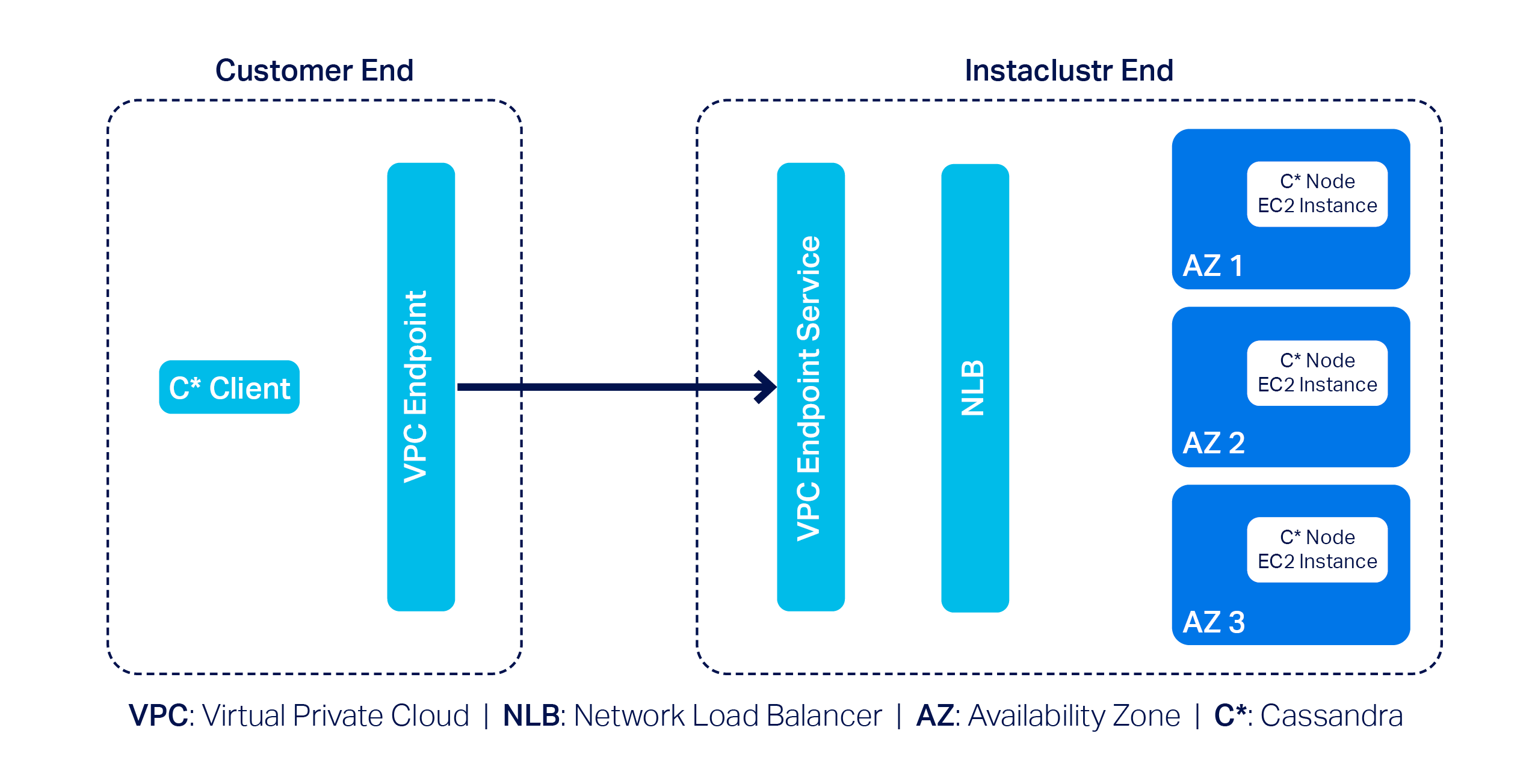
In this example, we have a 3-node Cassandra cluster at the far right with one Cassandra node per Availability Zone (or AZ). Next, we have the VPC Endpoint Service and a Network Load Balancer (NLB). The Endpoint Service is essentially the AWS PrivateLink, and by design AWS needs it to be backed by an NLB–that’s pretty much what we have to manage on our side.
On the customer side, they must create a VPC Endpoint that enables them to privately connect to the AWS PrivateLink on our end; naturally, customers will also have to use a Cassandra client(s) to connect to the cluster.
AWS PrivateLink support with Instaclustr for Apache Cassandra
To incorporate AWS PrivateLink support with Instaclustr for Apache Cassandra on our platform, we came across a few technical challenges. First and foremost, the primary challenge was relatively straightforward: Cassandra clients need to talk to each individual node in a cluster.
However, the problem is that nodes in an AWS PrivateLink cluster are only assigned private IPs; that is what the nodes would announce by default when Cassandra clients attempt to discover the topology of the cluster. Cassandra clients cannot do much with the received private IPs as they cannot be used to connect to the nodes directly in an AWS PrivateLink setup.
We devised a plan of attack to get around this problem:
- Make each individual Cassandra node listen for CQL queries on unique ports.
- Configure the NLB so it can route traffic to the appropriate node based on the relevant unique port.
- Let clients implement the AddressTranslator interface from the Cassandra driver. The custom address translator will need to translate the received private IPs to one of the VPC Endpoint Elastic Network Interface (or ENI) IPs without altering the corresponding unique ports.
To understand this approach better, consider the following example:
Suppose we have a 3-node Cassandra cluster. According to the proposed approach we will need to do the followings:
- Let the nodes listen on ports 172.16.0.1:6001 (in AZ1), 172.16.0.2: 6002 (in AZ2) and 172.16.0.3: 6003 (in AZ3)
- Configure the NLB to listen on the same set of ports
- Define and associate target groups based on the port. For instance, the listener on port 6002 will be associated with a target group containing only the node that is listening on port 6002.
- As for how the custom address translator is expected to work,
let’s assume the VPC Endpoint ENI IPs are 192.168.0.1 (in AZ1),
192.168.0.2 (in AZ2) and 192.168.0.3 (in AZ3). The address
translator should translate received addresses like so:
- 172.16.0.1:6001 --> 192.168.0.1:6001
- 172.16.0.2:6002 --> 192.168.0.2:6002
- 172.16.0.3:6003 --> 192.168.0.3:6003
The proposed approach not only solves the connectivity problem but also allows for connecting to appropriate nodes based on query plans generated by load balancing policies.
Around the same time, we came up with a slightly modified approach as well: we realized the need for address translation can be mostly mitigated if we make the Cassandra nodes return the VPC Endpoint ENI IPs in the first place.
But the excitement did not last for long! Why? Because we quickly discovered a key problem: there is a limit to the number of listeners that can be added to any given AWS NLB of just 50.
While 50 is certainly a decent limit, the way we designed our solution meant we wouldn’t be able to provision a cluster with more than 50 nodes. This was quickly deemed to be an unacceptable limitation as it is not uncommon for a cluster to have more than 50 nodes; many Cassandra clusters in our fleet have hundreds of nodes. We had to abandon the idea of address translation and started thinking about alternative solution approaches.
Introducing Shotover Proxy
We were disappointed but did not lose hope. Soon after, we devised a practical solution centred around using one of our open source products: Shotover Proxy.
Shotover Proxy is used with Cassandra clusters to support AWS PrivateLink on the Instaclustr Managed Platform. What is Shotover Proxy, you ask? Shotover is a layer 7 database proxy built to allow developers, admins, DBAs, and operators to modify in-flight database requests. By managing database requests in transit, Shotover gives NetApp Instaclustr customers AWS PrivateLink’s simple and secure network setup with the many benefits of Cassandra.
Below is an updated version of the previous diagram that introduces some Shotover nodes in the mix:
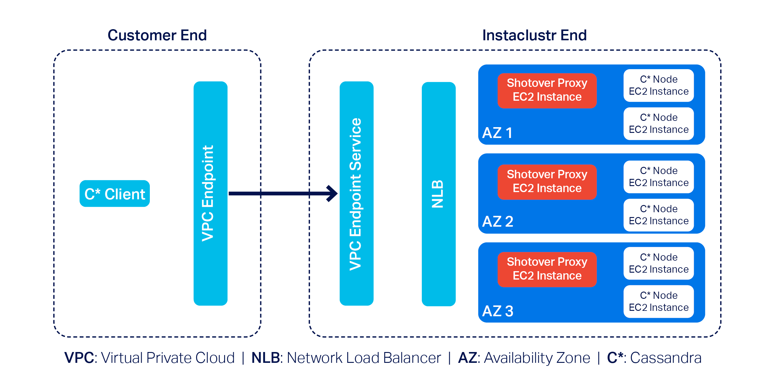
As you can see, each AZ now has a dedicated Shotover proxy node.
In the above diagram, we have a 6-node Cassandra cluster. The Cassandra cluster sitting behind the Shotover nodes is an ordinary Private Network Cluster. The role of the Shotover nodes is to manage client requests to the Cassandra nodes while masking the real Cassandra nodes behind them. To the Cassandra client, the Shotover nodes appear to be Cassandra nodes, and it is only them that make up the entire cluster! This is the secret recipe for AWS PrivateLink for Instaclustr for Apache Cassandra that enabled us to get past the challenges discussed earlier.
So how is this model made to work?
Shotover can alter certain requests from—and responses to—the client. It can examine the tokens allocated to the Cassandra nodes in its own AZ (aka rack) and claim to be the owner of all those tokens. This essentially makes them appear to be an aggregation of the nodes in its own rack.
Given the purposely crafted topology and token allocation metadata, while the client directs queries to the Shotover node, the Shotover node in turn can pass them on to the appropriate Cassandra node and then transparently send responses back. It is worth noting that the Shotover nodes themselves do not store any data.
Because we only have 1 Shotover node per AZ in this design and there may be at most about 5 AZs per region, we only need that many listeners in the NLB to make this mechanism work. As such, the 50-listener limit on the NLB was no longer a problem.
The use of Shotover to manage client driver and cluster interoperability may sound straight forward to implement, but developing it was a year-long undertaking. As described above, the initial months of development were devoted to engineering CQL queries on unique ports and the AddressTranslator interface from the Cassandra driver to gracefully manage client connections to the Cassandra cluster. While this solution did successfully provide support for AWS PrivateLink with a Cassandra cluster, we knew that the 50-listener limit on the NLB was a barrier for use and wanted to provide our customers with a solution that could be used for any Cassandra cluster, regardless of node count.
The next few months of engineering were then devoted to the Proof of Concept of an alternative solution with the goal to investigate how Shotover could manage client requests for a Cassandra cluster with any number of nodes. And so, after a solution to support a cluster with any number of nodes was successfully proved, subsequent effort was then devoted to work through stability testing the new solution, the results of that engineering being the stable solution described above.
We have also conducted performance testing to evaluate the relative performance of a PrivateLink-enabled Cassandra cluster compared to its non-PrivateLink counterpart. Multiple iterations of performance testing were executed as some adjustments to Shotover were identified from test cases and resulted in the PrivateLink-enabled Cassandra cluster throughput and latency measuring near to a standard Cassandra cluster throughput and latency.
Related content: Read more about creating an AWS PrivateLink-enabled Cassandra cluster on the Instaclustr Managed Platform
The following was our experimental setup for identifying the max throughput in terms of Operations per second of a Cassandra PrivateLink cluster in comparison to a non-Cassandra PrivateLink cluster
- Baseline node size:
i3en.xlarge - Shotover Proxy node size on Cassandra Cluster:
CSO-PRD-c6gd.medium-54 - Cassandra version:
4.1.3 - Shotover Proxy version:
0.2.0 - Other configuration: Repair and backup disabled, Client Encryption disabled
Throughput results
| Operation | Operation rate with PrivateLink and Shotover | Operation rate without PrivateLink |
| Mixed-small (3 Nodes) | 16608 | 16206 |
| Mixed-small (6 Nodes) | 33585 | 33598 |
| Mixed-small (9 Nodes) | 51792 | 51798 |
Across different cluster sizes, we observed no significant difference in operation throughput between PrivateLink and non-PrivateLink configurations.
Latency results
Latency benchmarks were conducted at ~70% of the observed peak throughput (as above) to simulate realistic production traffic.
| Operation | Ops/second | Setup | Mean Latency (ms) | Median Latency (ms) | P95 Latency (ms) | P99 Latency (ms) |
| Mixed-small (3 Nodes) | 11630 | Non-PrivateLink | 9.90 | 3.2 | 53.7 | 119.4 |
| PrivateLink | 9.50 | 3.6 | 48.4 | 118.8 | ||
| Mixed-small (6 Nodes) | 23510 | Non-PrivateLink | 6 | 2.3 | 27.2 | 79.4 |
| PrivateLink | 9.10 | 3.4 | 45.4 | 104.9 | ||
| Mixed-small (9 Nodes) | 36255 | Non-PrivateLink | 5.5 | 2.4 | 21.8 | 67.6 |
| PrivateLink | 11.9 | 2.7 | 77.1 | 141.2 |
Results indicate that for lower to mid-tier throughput levels, AWS PrivateLink introduced minimal to negligible overhead. However, at higher operation rates, we observed increased latency, most notably at the p99 mark—likely due to network level factors or Shotover.
The increase in latency is expected as AWS PrivateLink introduces an additional hop to route traffic securely, which can impact latencies, particularly under heavy load. For the vast majority of applications, the observed latencies remain within acceptable ranges. However, for latency-sensitive workloads, we recommend adding more nodes (for high load cases) to help mitigate the impact of the additional network hop introduced by PrivateLink.
As with any generic benchmarking results, performance may vary depending on specific data model, workload characteristics, and environment. The results presented here are based on specific experimental setup using standard configurations and should primarily be used to compare the relative performance of PrivateLink vs. Non-PrivateLink networking under similar conditions.
Why choose AWS PrivateLink with NetApp Instaclustr?
NetApp’s commitment to innovation means you benefit from cutting-edge technology combined with ease of use. With AWS PrivateLink support on our platform, customers gain:
- Enhanced security: All traffic stays private, never touching the internet.
- Simplified networking: No need to manage complex CIDR overlaps.
- Enterprise scalability: Handles sizable clusters effortlessly.
By addressing challenges, such as the NLB listener cap and private-to-VPC IP translation, we’ve created a solution that balances efficiency, security, and scalability.
Experience PrivateLink today
The integration of AWS PrivateLink with Apache Cassandra® is now generally available with production-ready SLAs for our customers. Log in to the Console to create a Cassandra cluster with support for AWS PrivateLink with just a few clicks today. Whether you’re managing sensitive workloads or demanding performance at scale, this feature delivers unmatched value.
Want to see it in action? Book a free demo today and experience the Shotover-powered magic of AWS PrivateLink firsthand.
Resources
- Getting started: Visit the documentation to learn how to create an AWS PrivateLink-enabled Apache Cassandra cluster on the Instaclustr Managed Platform.
- Connecting clients: Already created a Cassandra cluster with AWS PrivateLink? Click here to read about how to connect Cassandra clients in one VPC to an AWS PrivateLink-enabled Cassandra cluster on the Instaclustr Platform.
- General availability announcement: For more details, read our General Availability announcement on AWS PrivateLink support for Cassandra.
The post Integrating support for AWS PrivateLink with Apache Cassandra® on the NetApp Instaclustr Managed Platform appeared first on Instaclustr.
Compaction Strategies, Performance, and Their Impact on Cassandra Node Density
This is the third post in my series on optimizing Apache Cassandra for maximum cost efficiency through increased node density. In the first post, I examined how streaming operations impact node density and laid out the groundwork for understanding why higher node density leads to significant cost savings. In the second post, I discussed how compaction throughput is critical to node density and introduced the optimizations we implemented in CASSANDRA-15452 to improve throughput on disaggregated storage like EBS.
Cassandra Compaction Throughput Performance Explained
This is the second post in my series on improving node density and lowering costs with Apache Cassandra. In the previous post, I examined how streaming performance impacts node density and operational costs. In this post, I’ll focus on compaction throughput, and a recent optimization in Cassandra 5.0.4 that significantly improves it, CASSANDRA-15452.
This post assumes some familiarity with Apache Cassandra storage engine fundamentals. The documentation has a nice section covering the storage engine if you’d like to brush up before reading this post.
CEP-24 Behind the scenes: Developing Apache Cassandra®’s password validator and generator
Introduction: The need for an Apache Cassandra® password validator and generator
Here’s the problem: while users have always had the ability to create whatever password they wanted in Cassandra–from straightforward to incredibly complex and everything in between–this ultimately created a noticeable security vulnerability.
While organizations might have internal processes for generating secure passwords that adhere to their own security policies, Cassandra itself did not have the means to enforce these standards. To make the security vulnerability worse, if a password initially met internal security guidelines, users could later downgrade their password to a less secure option simply by using “ALTER ROLE” statements.
When internal password requirements are enforced for an individual, users face the additional burden of creating compliant passwords. This inevitably involved lots of trial-and-error in attempting to create a compliant password that satisfied complex security roles.
But what if there was a way to have Cassandra automatically create passwords that meet all bespoke security requirements–but without requiring manual effort from users or system operators?
That’s why we developed CEP-24: Password validation/generation. We recognized that the complexity of secure password management could be significantly reduced (or eliminated entirely) with the right approach–and improving both security and user experience at the same time.
The Goals of CEP-24
A Cassandra Enhancement Proposal (or CEP) is a structured process for proposing, creating, and ultimately implementing new features for the Cassandra project. All CEPs are thoroughly vetted among the Cassandra community before they are officially integrated into the project.
These were the key goals we established for CEP-24:
- Introduce a way to enforce password strength upon role creation or role alteration.
- Implement a reference implementation of a password validator which adheres to a recommended password strength policy, to be used for Cassandra users out of the box.
- Emit a warning (and proceed) or just reject “create role” and “alter role” statements when the provided password does not meet a certain security level, based on user configuration of Cassandra.
- To be able to implement a custom password validator with its own policy, whatever it might be, and provide a modular/pluggable mechanism to do so.
- Provide a way for Cassandra to generate a password which would pass the subsequent validation for use by the user.
The Cassandra Password Validator and Generator builds upon an established framework in Cassandra called Guardrails, which was originally implemented under CEP-3 (more details here).
The password validator implements a custom guardrail introduced
as part of
CEP-24. A custom guardrail can validate and generate values of
arbitrary types when properly implemented. In the CEP-24 context,
the password guardrail provides
CassandraPasswordValidator by extending
ValueValidator, while passwords are generated by
CassandraPasswordGenerator by extending
ValueGenerator. Both components work with passwords as
String type values.
Password validation and generation are configured in the
cassandra.yaml file under the
password_validator section. Let’s explore the key
configuration properties available. First, the
class_name and generator_class_name
parameters specify which validator and generator classes will be
used to validate and generate passwords respectively.
Cassandra
ships CassandraPasswordValidator and CassandraPasswordGenerator out
of the box. However, if a particular enterprise decides that they
need something very custom, they are free to implement their own
validators, put it on Cassandra’s class path and reference it in
the configuration behind class_name parameter. Same for the
validator.
CEP-24 provides implementations of the validator and generator that the Cassandra team believes will satisfy the requirements of most users. These default implementations address common password security needs. However, the framework is designed with flexibility in mind, allowing organizations to implement custom validation and generation rules that align with their specific security policies and business requirements.
password_validator:
 # Implementation class of a validator. When not in form of FQCN, the
 # package name org.apache.cassandra.db.guardrails.validators is prepended.
 # By default, there is no validator.
 class_name: CassandraPasswordValidator
 # Implementation class of related generator which generates values which are valid when
 # tested against this validator. When not in form of FQCN, the
 # package name org.apache.cassandra.db.guardrails.generators is prepended.
 # By default, there is no generator.
 generator_class_name: CassandraPasswordGenerator
Password quality might be looked at as the number of characteristics a password satisfies. There are two levels for any password to be evaluated – warning level and failure level. Warning and failure levels nicely fit into how Guardrails act. Every guardrail has warning and failure thresholds. Based on what value a specific guardrail evaluates, it will either emit a warning to a user that its usage is discouraged (but ultimately allowed) or it will fail to be set altogether.
This same principle applies to password evaluation – each password is assessed against both warning and failure thresholds. These thresholds are determined by counting the characteristics present in the password. The system evaluates five key characteristics: the password’s overall length, the number of uppercase characters, the number of lowercase characters, the number of special characters, and the number of digits. A comprehensive password security policy can be enforced by configuring minimum requirements for each of these characteristics.
# There are four characteristics:
 # upper-case, lower-case, special character and digit.
 # If this value is set e.g. to 3, a password has to
 # consist of 3 out of 4 characteristics.

 # For example, it has to contain at least 2 upper-case characters,
 # 2 lower-case, and 2 digits to pass,
 # but it does not have to contain any special characters.
 # If the number of characteristics found in the password is
 # less than or equal to this number, it will emit a warning.
 characteristic_warn: 3
 # If the number of characteristics found in the password is
 #less than or equal to this number, it will emit a failure.
 characteristic_fail: 2
Next, there are configuration parameters for each characteristic which count towards warning or failure:
# If the password is shorter than this value,
# the validator will emit a warning.
length_warn: 12
# If a password is shorter than this value,
# the validator will emit a failure.
length_fail: 8
# If a password does not contain at least n
# upper-case characters, the validator will emit a warning.
upper_case_warn: 2
# If a password does not contain at least
# n upper-case characters, the validator will emit a failure.
upper_case_fail: 1
# If a password does not contain at least
# n lower-case characters, the validator will emit a warning.
lower_case_warn: 2
# If a password does not contain at least
# n lower-case characters, the validator will emit a failure.
lower_case_fail: 1
# If a password does not contain at least
# n digits, the validator will emit a warning.
digit_warn: 2
# If a password does not contain at least
# n digits, the validator will emit a failure.
digit_fail: 1
# If a password does not contain at least
# n special characters, the validator will emit a warning.
special_warn: 2
# If a password does not contain at least
# n special characters, the validator will emit a failure.
special_fail: 1
It is also possible to say that illegal sequences of certain length found in a password will be forbidden:
# If a password contains illegal sequences that are at least this long, it is invalid.
# Illegal sequences might be either alphabetical (form 'abcde'),
# numerical (form '34567'), or US qwerty (form 'asdfg') as well
# as sequences from supported character sets.
# The minimum value for this property is 3,
# by default it is set to 5.
illegal_sequence_length: 5
Lastly, it is also possible to configure a dictionary of passwords to check against. That way, we will be checking against password dictionary attacks. It is up to the operator of a cluster to configure the password dictionary:
# Dictionary to check the passwords against. Defaults to no dictionary.
# Whole dictionary is cached into memory. Use with caution with relatively big dictionaries.
# Entries in a dictionary, one per line, have to be sorted per String's compareTo contract.
dictionary: /path/to/dictionary/file
Now that we have gone over all the configuration parameters, let’s take a look at an example of how password validation and generation look in practice.
Consider a scenario where a Cassandra super-user (such as the default ‘cassandra’ role) attempts to create a new role named ‘alice’.
cassandra@cqlsh> CREATE ROLE alice WITH PASSWORD = 'cassandraisadatabase' AND LOGIN = true;

InvalidRequest: Error from server: code=2200 [Invalid query]
message="Password was not set as it violated configured password strength
policy. To fix this error, the following has to be resolved: Password
contains the dictionary word 'cassandraisadatabase'. You may also use
'GENERATED PASSWORD' upon role creation or alteration."
The password is not found in the dictionary, but it is not long enough. When an operator sees this, they will try to fix it by making the password longer:
cassandra@cqlsh> CREATE ROLE alice WITH PASSWORD = 'T8aum3?' AND LOGIN = true;
InvalidRequest: Error from server: code=2200 [Invalid query]
message="Password was not set as it violated configured password strength
policy. To fix this error, the following has to be resolved: Password
must be 8 or more characters in length. You may also use
'GENERATED PASSWORD' upon role creation or alteration."
The password is finally set, but it is not completely secure. It satisfies the minimum requirements but our validator identified that not all characteristics were met.
cassandra@cqlsh> CREATE ROLE alice WITH PASSWORD = 'mYAtt3mp' AND LOGIN = true;

Warnings:

Guardrail password violated: Password was set, however it might not be
strong enough according to the configured password strength policy.
To fix this warning, the following has to be resolved: Password must be 12 or more
characters in length. Passwords must contain 2 or more digit characters. Password
must contain 2 or more special characters. Password matches 2 of 4 character rules,
but 4 are required. You may also use 'GENERATED PASSWORD' upon role creation or alteration.
The password is finally set, but it is not completely secure. It satisfies the minimum requirements but our validator identified that not all characteristics were met.
When an operator saw this, they noticed the note about the ‘GENERATED PASSWORD’ clause which will generate a password automatically without an operator needing to invent it on their own. This is a lot of times, as shown, a cumbersome process better to be left on a machine. Making it also more efficient and reliable.
cassandra@cqlsh> ALTER ROLE alice WITH GENERATED PASSWORD;

generated_password
------------------
   R7tb33?.mcAX
The generated password shown above will satisfy all the rules we have configured in the cassandra.yaml automatically. Every generated password will satisfy all of the rules. This is clearly an advantage over manual password generation.
When the CQL statement is executed, it will be visible in the CQLSH history (HISTORY command or in cqlsh_history file) but the password will not be logged, hence it cannot leak. It will also not appear in any auditing logs. Previously, Cassandra had to obfuscate such statements. This is not necessary anymore.
We can create a role with generated password like this:
cassandra@cqlsh> CREATE ROLE alice WITH GENERATED PASSWORD AND LOGIN = true;

or by CREATE USER:

cassandra@cqlsh> CREATE USER alice WITH GENERATED PASSWORD;
When a password is generated for alice (out of scope of this documentation), she can log in:
$ cqlsh -u alice -p R7tb33?.mcAX
...
alice@cqlsh>
Note: It is recommended to save password to ~/.cassandra/credentials, for example:
[PlainTextAuthProvider]
username = cassandra
password = R7tb33?.mcAX
and by setting auth_provider in ~/.cassandra/cqlshrc
[auth_provider]
module = cassandra.auth
classname = PlainTextAuthProvider
It is also possible to configure password validators in such a way that a user does not see why a password failed. This is driven by configuration property for password_validator called detailed_messages. When set to false, the violations will be very brief:
alice@cqlsh> ALTER ROLE alice WITH PASSWORD = 'myattempt';

InvalidRequest: Error from server: code=2200 [Invalid query]
message="Password was not set as it violated configured password strength policy.
You may also use 'GENERATED PASSWORD' upon role creation or alteration."
The following command will automatically generate a new password that meets all configured security requirements.
alice@cqlsh> ALTER ROLE alice WITH GENERATED PASSWORD;
Several potential enhancements to password generation and validation could be implemented in future releases. One promising extension would be validating new passwords against previous values. This would prevent users from reusing passwords until after they’ve created a specified number of different passwords. A related enhancement could include restricting how frequently users can change their passwords, preventing rapid cycling through passwords to circumvent history-based restrictions.
These features, while valuable for comprehensive password security, were considered beyond the scope of the initial implementation and may be addressed in future updates.
Final thoughts and next steps
The Cassandra Password Validator and Generator implemented under CEP-24 represents a significant improvement in Cassandra’s security posture.
By providing robust, configurable password policies with built-in enforcement mechanisms and convenient password generation capabilities, organizations can now ensure compliance with their security standards directly at the database level. This not only strengthens overall system security but also improves the user experience by eliminating guesswork around password requirements.
As Cassandra continues to evolve as an enterprise-ready database solution, these security enhancements demonstrate a commitment to meeting the demanding security requirements of modern applications while maintaining the flexibility that makes Cassandra so powerful.
Ready to experience CEP-24 yourself? Try it out on the Instaclustr Managed Platform and spin up your first Cassandra cluster for free.
CEP-24 is just our latest contribution to open source. Check out everything else we’re working on here.
The post CEP-24 Behind the scenes: Developing Apache Cassandra®’s password validator and generator appeared first on Instaclustr.
Introduction to similarity search: Part 2–Simplifying with Apache Cassandra® 5’s new vector data type
In Part 1 of this series, we explored how you can combine Cassandra 4 and OpenSearch to perform similarity searches with word embeddings. While that approach is powerful, it requires managing two different systems.
But with the release of Cassandra 5, things become much simpler.
Cassandra 5 introduces a native VECTOR data type and built-in Vector Search capabilities, simplifying the architecture by enabling Cassandra 5 to handle storage, indexing, and querying seamlessly within a single system.
Now in Part 2, we’ll dive into how Cassandra 5 streamlines the process of working with word embeddings for similarity search. We’ll walk through how the new vector data type works, how to store and query embeddings, and how the Storage-Attached Indexing (SAI) feature enhances your ability to efficiently search through large datasets.
The power of vector search in Cassandra 5
Vector search is a game-changing feature added in Cassandra 5 that enables you to perform similarity searches directly within the database. This is especially useful for AI applications, where embeddings are used to represent data like text or images as high-dimensional vectors. The goal of vector search is to find the closest matches to these vectors, which is critical for tasks like product recommendations or image recognition.
The key to this functionality lies in embeddings: arrays of floating-point numbers that represent the similarity of objects. By storing these embeddings as vectors in Cassandra, you can use Vector Search to find connections in your data that may not be obvious through traditional queries.
How vectors work
Vectors are fixed-size sequences of non-null values, much like lists. However, in Cassandra 5, you cannot modify individual elements of a vector — you must replace the entire vector if you need to update it. This makes vectors ideal for storing embeddings, where you need to work with the whole data structure at once.
When working with embeddings, you’ll typically store them as vectors of floating-point numbers to represent the semantic meaning.
Storage-Attached Indexing (SAI): The engine behind vector search
Vector Search in Cassandra 5 is powered by Storage-Attached Indexing, which enables high-performance indexing and querying of vector data. SAI is essential for Vector Search, providing the ability to create column-level indexes on vector data types. This ensures that your vector queries are both fast and scalable, even with large datasets.
SAI isn’t just limited to vectors—it also indexes other types of data, making it a versatile tool for boosting the performance of your queries across the board.
Example: Performing similarity search with Cassandra 5’s vector data type
Now that we’ve introduced the new vector data type and the power of Vector Search in Cassandra 5, let’s dive into a practical example. In this section, we’ll show how to set up a table to store embeddings, insert data, and perform similarity searches directly within Cassandra.
Step 1: Setting up the embeddings table
To get started with this example, you’ll need access to a Cassandra 5 cluster. Cassandra 5 introduces native support for vector data types and Vector Search, available on Instaclustr’s managed platform. Once you have your cluster up and running, the first step is to create a table to store the embeddings. We’ll also create an index on the vector column to optimize similarity searches using SAI.
CREATE KEYSPACE aisearch WITH REPLICATION = {{'class': 'SimpleStrategy',         '       replication_factor': 1}};


CREATE TABLE IF NOT EXISTS embeddings (
    id UUID,
    paragraph_uuid UUID,
    filename TEXT,
    embeddings vector<float, 300>,
    text TEXT,
    last_updated timestamp,
    PRIMARY KEY (id, paragraph_uuid)
);


CREATE INDEX IF NOT EXISTS ann_index
  ON embeddings(embeddings) USING 'sai';
This setup allows us to store the embeddings as 300-dimensional vectors, along with metadata like file names and text. The SAI index will be used to speed up similarity searches on the embedding’s column.
You can also fine-tune the index by specifying the similarity function to be used for vector comparisons. Cassandra 5 supports three types of similarity functions: DOT_PRODUCT, COSINE, and EUCLIDEAN. By default, the similarity function is set to COSINE, but you can specify your preferred method when creating the index:
CREATE INDEX IF NOT EXISTS ann_index
    ON embeddings(embeddings) USING 'sai'
WITH OPTIONS = { 'similarity_function': 'DOT_PRODUCT' };
Each similarity function has its own advantages depending on your use case. DOT_PRODUCT is often used when you need to measure the direction and magnitude of vectors, COSINE is ideal for comparing the angle between vectors, and EUCLIDEAN calculates the straight-line distance between vectors. By selecting the appropriate function, you can optimize your search results to better match the needs of your application.
Step 2: Inserting embeddings into Cassandra 5
To insert embeddings into Cassandra 5, we can use the same code from the first part of this series to extract text from files, load the FastText model, and generate the embeddings. Once the embeddings are generated, the following function will insert them into Cassandra:
import time
from uuid import uuid4, UUID
from cassandra.cluster import Cluster
from cassandra.query import SimpleStatement
from cassandra.policies import DCAwareRoundRobinPolicy
from cassandra.auth import PlainTextAuthProvider
from google.colab import userdata

# Connect to the single-node cluster
cluster = Cluster(
# Replace with your IP list
["xxx.xxx.xxx.xxx", "xxx.xxx.xxx.xxx ", " xxx.xxx.xxx.xxx "], # Single-node cluster address
load_balancing_policy=DCAwareRoundRobinPolicy(local_dc='AWS_VPC_US_EAST_1'), # Update the local data centre if needed
port=9042,
auth_provider=PlainTextAuthProvider (
username='iccassandra',
password='replace_with_your_password'
)
)
session = cluster.connect()

print('Connected to cluster %s' % cluster.metadata.cluster_name)

def insert_embedding_to_cassandra(session, embedding, id=None, paragraph_uuid=None, filename=None, text=None, keyspace_name=None):
try:
embeddings = list(map(float, embedding))

# Generate UUIDs if not provided
if id is None:
id = uuid4()
if paragraph_uuid is None:
paragraph_uuid = uuid4()
# Ensure id and paragraph_uuid are UUID objects
if isinstance(id, str):
id = UUID(id)
if isinstance(paragraph_uuid, str):
paragraph_uuid = UUID(paragraph_uuid)

# Create the query string with placeholders
insert_query = f"""
INSERT INTO {keyspace_name}.embeddings (id, paragraph_uuid, filename, embeddings, text, last_updated)
VALUES (?, ?, ?, ?, ?, toTimestamp(now()))
"""

# Create a prepared statement with the query
prepared = session.prepare(insert_query)

# Execute the query
session.execute(prepared.bind((id, paragraph_uuid, filename, embeddings, text)))

return None # Successful insertion

except Exception as e:
error_message = f"Failed to execute query:\nError: {str(e)}"
return error_message # Return error message on failure

def insert_with_retry(session, embedding, id=None, paragraph_uuid=None,
filename=None, text=None, keyspace_name=None, max_retries=3,
retry_delay_seconds=1):
retry_count = 0
while retry_count < max_retries:
result = insert_embedding_to_cassandra(session, embedding, id, paragraph_uuid, filename, text, keyspace_name)
if result is None:
return True # Successful insertion
else:
retry_count += 1
print(f"Insertion failed on attempt {retry_count} with error: {result}")
if retry_count < max_retries:
time.sleep(retry_delay_seconds) # Delay before the next retry
return False # Failed after max_retries

# Replace the file path pointing to the desired file
file_path = "/path/to/Cassandra-Best-Practices.pdf"
paragraphs_with_embeddings =
extract_text_with_page_number_and_embeddings(file_path)

from tqdm import tqdm

for paragraph in tqdm(paragraphs_with_embeddings, desc="Inserting paragraphs"):
if not insert_with_retry(
session=session,
embedding=paragraph['embedding'],
id=paragraph['uuid'],
paragraph_uuid=paragraph['paragraph_uuid'],
text=paragraph['text'],
filename=paragraph['filename'],
keyspace_name=keyspace_name,
max_retries=3,
retry_delay_seconds=1
):
# Display an error message if insertion fails
tqdm.write(f"Insertion failed after maximum retries for UUID
{paragraph['uuid']}: {paragraph['text'][:50]}...")
This function handles inserting embeddings and metadata into Cassandra, ensuring that UUIDs are correctly generated for each entry.
Step 3: Performing similarity searches in Cassandra 5
Once the embeddings are stored, we can perform similarity searches directly within Cassandra using the following function:
import numpy as np
# ------------------ Embedding Functions ------------------
def text_to_vector(text):
"""Convert a text chunk into a vector using the FastText model."""
words = text.split()
vectors = [fasttext_model[word] for word in words if word in fasttext_model.key_to_index]
return np.mean(vectors, axis=0) if vectors else np.zeros(fasttext_model.vector_size)

def find_similar_texts_cassandra(session, input_text, keyspace_name=None, top_k=5):
# Convert the input text to an embedding
input_embedding = text_to_vector(input_text)
input_embedding_str = ', '.join(map(str, input_embedding.tolist()))

# Adjusted query without the ORDER BY clause and correct comment syntax
query = f"""
SELECT text, filename, similarity_cosine(embeddings, ?) AS similarity
FROM {keyspace_name}.embeddings
ORDER BY embeddings ANN OF [{input_embedding_str}]
LIMIT {top_k};
"""

prepared = session.prepare(query)
bound = prepared.bind((input_embedding,))
rows = session.execute(bound)

# Sort the results by similarity in Python
similar_texts = sorted([(row.similarity, row.filename, row.text) for row in rows], key=lambda x: x[0], reverse=True)

return similar_texts[:top_k]

from IPython.display import display, HTML

# The word you want to find similarities for
input_text = "place"

# Call the function to find similar texts in the Cassandra database
similar_texts = find_similar_texts_cassandra(session, input_text, keyspace_name="aisearch", top_k=10)
This function searches for similar embeddings in Cassandra and retrieves the top results based on cosine similarity. Under the hood, Cassandra’s vector search uses Hierarchical Navigable Small Worlds (HNSW). HNSW organizes data points in a multi-layer graph structure, making queries significantly faster by narrowing down the search space efficiently—particularly important when handling large datasets.
Step 4: Displaying the results
To display the results in a readable format, we can loop through the similar texts and present them along with their similarity scores:
# Print the similar texts along with their similarity scores
for similarity, filename, text in similar_texts:
html_content = f"""
<div style="margin-bottom: 10px;">
<p><b>Similarity:</b> {similarity:.4f}</p>
<p><b>Text:</b> {text}</p>
<p><b>File:</b> {filename}</p>
</div>
<hr/>
"""

display(HTML(html_content))
This code will display the top similar texts, along with their similarity scores and associated file names.
Cassandra 5 vs. Cassandra 4 + OpenSearch®
Cassandra 4 relies on an integration with OpenSearch to handle word embeddings and similarity searches. This approach works well for applications that are already using or comfortable with OpenSearch, but it does introduce additional complexity with the need to maintain two systems.
Cassandra 5, on the other hand, brings vector support directly into the database. With its native VECTOR data type and similarity search functions, it simplifies your architecture and improves performance, making it an ideal solution for applications that require embedding-based searches at scale.
| Feature | Cassandra 4 + OpenSearch | Cassandra 5 (Preview) |
| Embedding Storage | OpenSearch | Native VECTOR Data Type |
| Similarity Search | KNN Plugin in OpenSearch | COSINE, EUCLIDEAN, DOT_PRODUCT |
| Search Method | Exact K-Nearest Neighbor | Approximate Nearest Neighbor (ANN) |
| System Complexity | Requires two systems | All-in-one Cassandra solution |
Conclusion: A simpler path to similarity search with Cassandra 5
With Cassandra 5, the complexity of setting up and managing a separate search system for word embeddings is gone. The new vector data type and Vector Search capabilities allow you to perform similarity searches directly within Cassandra, simplifying your architecture and making it easier to build AI-powered applications.
Coming up: more in-depth examples and use cases that demonstrate how to take full advantage of these new features in Cassandra 5 in future blogs!
Ready to experience vector search with Cassandra 5? Spin up your first cluster for free on the Instaclustr Managed Platform and try it out!
The post Introduction to similarity search: Part 2–Simplifying with Apache Cassandra® 5’s new vector data type appeared first on Instaclustr.
Introduction to similarity search with word embeddings: Part 1–Apache Cassandra® 4.0 and OpenSearch®
Word embeddings have revolutionized how we approach tasks like natural language processing, search, and recommendation engines.
They allow us to convert words and phrases into numerical representations (vectors) that capture their meaning based on the context in which they appear. Word embeddings are especially useful for tasks where traditional keyword searches fall short, such as finding semantically similar documents or making recommendations based on textual data.

For example: a search for “Laptop” might return results related to “Notebook” or “MacBook” when using embeddings (as opposed to something like “Tablet”) offering a more intuitive and accurate search experience.
As applications increasingly rely on AI and machine learning to drive intelligent search and recommendation engines, the ability to efficiently handle word embeddings has become critical. That’s where databases like Apache Cassandra come into play—offering the scalability and performance needed to manage and query large amounts of vector data.
In Part 1 of this series, we’ll explore how you can leverage word embeddings for similarity searches using Cassandra 4 and OpenSearch. By combining Cassandra’s robust data storage capabilities with OpenSearch’s powerful search functions, you can build scalable and efficient systems that handle both metadata and word embeddings.
Cassandra 4 and OpenSearch: A partnership for embeddings
Cassandra 4 doesn’t natively support vector data types or specific similarity search functions, but that doesn’t mean you’re out of luck. By integrating Cassandra with OpenSearch, an open-source search and analytics platform, you can store word embeddings and perform similarity searches using the k-Nearest Neighbors (kNN) plugin.
This hybrid approach is advantageous over relying on OpenSearch alone because it allows you to leverage Cassandra’s strengths as a high-performance, scalable database for data storage while using OpenSearch for its robust indexing and search capabilities.
Instead of duplicating large volumes of data into OpenSearch solely for search purposes, you can keep the original data in Cassandra. OpenSearch, in this setup, acts as an intelligent pointer, indexing the embeddings stored in Cassandra and performing efficient searches without the need to manage the entire dataset directly.
This approach not only optimizes resource usage but also enhances system maintainability and scalability by segregating storage and search functionalities into specialized layers.
Deploying the environment
To set up your environment for word embeddings and similarity search, you can leverage the Instaclustr Managed Platform, which simplifies deploying and managing your Cassandra cluster and OpenSearch. Instaclustr takes care of the heavy lifting, allowing you to focus on building your application rather than managing infrastructure. In this configuration, Cassandra serves as your primary data store, while OpenSearch handles vector operations and similarity searches.
Here’s how to get started:
- Deploy a managed Cassandra cluster: Start by provisioning your Cassandra 4 cluster on the Instaclustr platform. This managed solution ensures your cluster is optimized, secure, and ready to store non-vector data.
- Set up OpenSearch with kNN plugin: Instaclustr also offers a fully managed OpenSearch service. You will need to deploy OpenSearch, with the kNN plugin enabled, which is critical for handling word embeddings and executing similarity searches.
By using Instaclustr, you gain access to a robust platform that seamlessly integrates Cassandra and OpenSearch, combining Cassandra’s scalable, fault-tolerant database with OpenSearch’s powerful search capabilities. This managed environment minimizes operational complexity, so you can focus on delivering fast and efficient similarity searches for your application.
Preparing the environment
Now that we’ve outlined the environment setup, let’s dive into the specific technical steps to prepare Cassandra and OpenSearch for storing and searching word embeddings.
Step 1: Setting up Cassandra
In Cassandra, we’ll need to create a table to store the metadata. Here’s how to do that:
- Create the Table:
Next, create a table to store the embeddings. This table will hold details such as the embedding vector, related text, and metadata:CREATE KEYSPACE IF NOT EXISTS aisearch WITH REPLICATION = {‘class’: ‘SimpleStrategy’, ‘
CREATE KEYSPACE IF NOT EXISTS aisearch WITH REPLICATION = {'class': 'SimpleStrategy',          '
replication_factor': 3};

USE file_metadata;

DROP TABLE IF EXISTS file_metadata;
    CREATE TABLE IF NOT EXISTS file_metadata (
      id UUID,
      paragraph_uuid UUID,
      filename TEXT,
      text TEXT,
      last_updated timestamp,
      PRIMARY KEY (id, paragraph_uuid)
    );
Step 2: Configuring OpenSearch
In OpenSearch, you’ll need to create an index that supports vector operations for similarity search. Here’s how you can configure it:
- Create the index:
Define the index settings and mappings, ensuring that vector operations are enabled and that the correct space type (e.g., L2) is used for similarity calculations.
{
  "settings": {
   "index": {
     "number_of_shards": 2,
      "knn": true,
      "knn.space_type": "l2"
    }
  },
  "mappings": {
    "properties": {
      "file_uuid": {
        "type": "keyword"
      },
      "paragraph_uuid": {
        "type": "keyword"
      },
      "embedding": {
        "type": "knn_vector",
        "dimension": 300
      }
    }
  }
}
This index configuration is optimized for storing and searching embeddings using the k-Nearest Neighbors algorithm, which is crucial for similarity search.
With these steps, your environment will be ready to handle word embeddings for similarity search using Cassandra and OpenSearch.
Generating embeddings with FastText
Once you have your environment set up, the next step is to generate the word embeddings that will drive your similarity search. For this, we’ll use FastText, a popular library from Facebook’s AI Research team that provides pre-trained word vectors. Specifically, we’re using the crawl-300d-2M model, which offers 300-dimensional vectors for millions of English words.
Step 1: Download and load the FastText model
To start, you’ll need to download the pre-trained model file. This can be done easily using Python and the requests library. Here’s the process:
1. Download the FastText model: The FastText model is stored in a zip file, which you can download from the official FastText website. The following Python script will handle the download and extraction:
import requests
import zipfile
import os

# Adjust file_url  and local_filename  variables accordingly
file_url = 'https://dl.fbaipublicfiles.com/fasttext/vectors-english/crawl-300d-2M.vec.zip'
local_filename = '/content/gdrive/MyDrive/0_notebook_files/model/crawl-300d-2M.vec.zip'
extract_dir = '/content/gdrive/MyDrive/0_notebook_files/model/'

def download_file(url, filename):
    with requests.get(url, stream=True) as r:
        r.raise_for_status()
        os.makedirs(os.path.dirname(filename), exist_ok=True)
        with open(filename, 'wb') as f:
            for chunk in r.iter_content(chunk_size=8192):
                f.write(chunk)


def unzip_file(filename, extract_to):
    with zipfile.ZipFile(filename, 'r') as zip_ref:
        zip_ref.extractall(extract_to)

# Download and extract
download_file(file_url, local_filename)
unzip_file(local_filename, extract_dir)
2. Load the model: Once the model is downloaded and extracted, you’ll load it using Gensim’s KeyedVectors class. This allows you to work with the embeddings directly:
from gensim.models import KeyedVectors

# Adjust model_path variable accordingly
model_path = "/content/gdrive/MyDrive/0_notebook_files/model/crawl-300d-2M.vec"
fasttext_model = KeyedVectors.load_word2vec_format(model_path, binary=False)
Step 2: Generate embeddings from text
With the FastText model loaded, the next task is to convert text into vectors. This process involves splitting the text into words, looking up the vector for each word in the FastText model, and then averaging the vectors to get a single embedding for the text.
Here’s a function that handles the conversion:
import numpy as np
import re

def text_to_vector(text):
    """Convert text into a vector using the FastText model."""
    text = text.lower()
    words = re.findall(r'\b\w+\b', text)
    vectors = [fasttext_model[word] for word in words if word in fasttext_model.key_to_index]

    if not vectors:
        print(f"No embeddings found for text: {text}")
        return np.zeros(fasttext_model.vector_size)

    return np.mean(vectors, axis=0)
This function tokenizes the input text, retrieves the corresponding word vectors from the model, and computes the average to create a final embedding.
Step 3: Extract text and generate embeddings from documents
In real-world applications, your text might come from various types of documents, such as PDFs, Word files, or presentations. The following code shows how to extract text from different file formats and convert that text into embeddings:
import uuid
import mimetypes
import pandas as pd
from pdfminer.high_level import extract_pages
from pdfminer.layout import LTTextContainer
from docx import Document
from pptx import Presentation

def generate_deterministic_uuid(name):
    return uuid.uuid5(uuid.NAMESPACE_DNS, name)

def generate_random_uuid():
    return uuid.uuid4()

def get_file_type(file_path):
    # Guess the MIME type based on the file extension
    mime_type, _ = mimetypes.guess_type(file_path)
    return mime_type

def extract_text_from_excel(excel_path):
    xls = pd.ExcelFile(excel_path)
    text_list = []

for sheet_index, sheet_name in enumerate(xls.sheet_names):
        df = xls.parse(sheet_name)
        for row in df.iterrows():
            text_list.append((" ".join(map(str, row[1].values)), sheet_index + 1))  # +1 to make it 1 based index

return text_list

def extract_text_from_pdf(pdf_path):
    return [(text_line.get_text().strip().replace('\xa0', ' '), page_num)
            for page_num, page_layout in enumerate(extract_pages(pdf_path), start=1)
            for element in page_layout if isinstance(element, LTTextContainer)
            for text_line in element if text_line.get_text().strip()]

def extract_text_from_word(file_path):
    doc = Document(file_path)
    return [(para.text, (i == 0) + 1) for i, para in enumerate(doc.paragraphs) if para.text.strip()]

def extract_text_from_txt(file_path):
    with open(file_path, 'r') as file:
        return [(line.strip(), 1) for line in file.readlines() if line.strip()]

def extract_text_from_pptx(pptx_path):
    prs = Presentation(pptx_path)
    return [(shape.text.strip(), slide_num) for slide_num, slide in enumerate(prs.slides, start=1)
            for shape in slide.shapes if hasattr(shape, "text") and shape.text.strip()]

def extract_text_with_page_number_and_embeddings(file_path, embedding_function):
    file_uuid = generate_deterministic_uuid(file_path)
    file_type = get_file_type(file_path)

    extractors = {
        'text/plain': extract_text_from_txt,
        'application/pdf': extract_text_from_pdf,
        'application/vnd.openxmlformats-officedocument.wordprocessingml.document': extract_text_from_word,
        'application/vnd.openxmlformats-officedocument.presentationml.presentation': extract_text_from_pptx,
        'application/zip': lambda path: extract_text_from_pptx(path) if path.endswith('.pptx') else [],
        'application/vnd.openxmlformats-officedocument.spreadsheetml.sheet': extract_text_from_excel,
        'application/vnd.ms-excel': extract_text_from_excel
    }

    text_list = extractors.get(file_type, lambda _: [])(file_path)

    return [
      {
          "uuid": file_uuid,
          "paragraph_uuid": generate_random_uuid(),
          "filename": file_path,
          "text": text,
          "page_num": page_num,
          "embedding": embedding
      }
      for text, page_num in text_list
      if (embedding := embedding_function(text)).any()  # Check if the embedding is not all zeros
    ]

# Replace the file path with the one you want to process

file_path = "../../docs-manager/Cassandra-Best-Practices.pdf"
paragraphs_with_embeddings = extract_text_with_page_number_and_embeddings(file_path)
This code handles extracting text from different document types, generating embeddings for each text chunk, and associating them with unique IDs.
With FastText set up and embeddings generated, you’re now ready to store these vectors in OpenSearch and start performing similarity searches.
Performing similarity searches
To conduct similarity searches, we utilize the k-Nearest Neighbors (kNN) plugin within OpenSearch. This plugin allows us to efficiently search for the most similar embeddings stored in the system. Essentially, you’re querying OpenSearch to find the closest matches to a word or phrase based on your embeddings.
For example, if you’ve embedded product descriptions, using kNN search helps you locate products that are semantically similar to a given input. This capability can significantly enhance your application’s recommendation engine, categorization, or clustering.
This setup with Cassandra and OpenSearch is a powerful combination, but it’s important to remember that it requires managing two systems. As Cassandra evolves, the introduction of built-in vector support in Cassandra 5 simplifies this architecture. But for now, let’s focus on leveraging both systems to get the most out of similarity searches.
Example: Inserting metadata in Cassandra and embeddings in OpenSearch
In this example, we use Cassandra 4 to store metadata related to files and paragraphs, while OpenSearch handles the actual word embeddings. By storing the paragraph and file IDs in both systems, we can link the metadata in Cassandra with the embeddings in OpenSearch.
We first need to store metadata such as the file name, paragraph UUID, and other relevant details in Cassandra. This metadata will be crucial for linking the data between Cassandra, OpenSearch and the file itself in filesystem.
The following code demonstrates how to insert this metadata into Cassandra and embeddings in OpenSearch, make sure to run the previous script, so the “paragraphs_with_embeddings” variable will be populated:
from tqdm import tqdm

# Function to insert data into both Cassandra and OpenSearch
def insert_paragraph_data(session, os_client, paragraph, keyspace_name, index_name):
    # Insert into Cassandra
    cassandra_result = insert_with_retry(
        session=session,
        id=paragraph['uuid'],
        paragraph_uuid=paragraph['paragraph_uuid'],
        text=paragraph['text'],
        filename=paragraph['filename'],
        keyspace_name=keyspace_name,
        max_retries=3,
        retry_delay_seconds=1
    )

    if not cassandra_result:
        return False  # Stop further processing if Cassandra insertion fails

    # Insert into OpenSearch
    opensearch_result = insert_embedding_to_opensearch(
        os_client=os_client,
        index_name=index_name,
        file_uuid=paragraph['uuid'],
        paragraph_uuid=paragraph['paragraph_uuid'],
        embedding=paragraph['embedding']
    )

    if opensearch_result is not None:
        return False  # Return False if OpenSearch insertion fails

    return True  # Return True on success for both

# Process each paragraph with a progress bar
print("Starting batch insertion of paragraphs.")

for paragraph in tqdm(paragraphs_with_embeddings, desc="Inserting paragraphs"):
    if not insert_paragraph_data(
        session=session,
        os_client=os_client,
        paragraph=paragraph,
        keyspace_name=keyspace_name,
        index_name=index_name
    ):

        print(f"Insertion failed for UUID {paragraph['uuid']}: {paragraph['text'][:50]}...")

print("Batch insertion completed.")
Performing similarity search
Now that we’ve stored both metadata in Cassandra and embeddings in OpenSearch, it’s time to perform a similarity search. This step involves searching OpenSearch for embeddings that closely match a given input and then retrieving the corresponding metadata from Cassandra.
The process is straightforward: we start by converting the input text into an embedding, then use the k-Nearest Neighbors (kNN) plugin in OpenSearch to find the most similar embeddings. Once we have the results, we fetch the related metadata from Cassandra, such as the original text and file name.
Here’s how it works:
- Convert text to embedding: Start by converting your input text into an embedding vector using the FastText model. This vector will serve as the query for our similarity search.
- Search OpenSearch for similar embeddings: Using the KNN search capability in OpenSearch, we find the top k most similar embeddings. Each result includes the corresponding file and paragraph UUIDs, which help us link the results back to Cassandra.
- Fetch metadata from Cassandra: With the UUIDs retrieved from OpenSearch, we query Cassandra to get the metadata, such as the original text and file name, associated with each embedding.
The following code demonstrates this process:
import uuid
from IPython.display import display, HTML

def find_similar_embeddings_opensearch(os_client, index_name, input_embedding, top_k=5):
    """Search for similar embeddings in OpenSearch and return the associated UUIDs."""
    query = {
        "size": top_k,
        "query": {
            "knn": {
                "embedding": {
                    "vector": input_embedding.tolist(),
                    "k": top_k
                }
            }
        }
    }

        response = os_client.search(index=index_name, body=query)

    similar_uuids = []
    for hit in response['hits']['hits']:
        file_uuid = hit['_source']['file_uuid']
        paragraph_uuid = hit['_source']['paragraph_uuid']
        similar_uuids.append((file_uuid, paragraph_uuid))

    return similar_uuids

def fetch_metadata_from_cassandra(session, file_uuid, paragraph_uuid, keyspace_name):
    """Fetch the metadata (text and filename) from Cassandra based on UUIDs."""
    file_uuid = uuid.UUID(file_uuid)
    paragraph_uuid = uuid.UUID(paragraph_uuid)

    query = f"""
    SELECT text, filename
    FROM {keyspace_name}.file_metadata
    WHERE id = ? AND paragraph_uuid = ?;
    """
    prepared = session.prepare(query)
    bound = prepared.bind((file_uuid, paragraph_uuid))
    rows = session.execute(bound)

    for row in rows:
        return row.filename, row.text
    return None, None

# Input text to find similar embeddings
input_text = "place"

# Convert input text to embedding
input_embedding = text_to_vector(input_text)

# Find similar embeddings in OpenSearch
similar_uuids = find_similar_embeddings_opensearch(os_client, index_name=index_name, input_embedding=input_embedding, top_k=10)

# Fetch and display metadata from Cassandra based on the UUIDs found in OpenSearch
for file_uuid, paragraph_uuid in similar_uuids:
    filename, text = fetch_metadata_from_cassandra(session, file_uuid, paragraph_uuid,
keyspace_name)

    if filename and text:
        html_content = f"""
        <div style="margin-bottom: 10px;">
            <p><b>File UUID:</b> {file_uuid}</p>
            <p><b>Paragraph UUID:</b> {paragraph_uuid}</p>
            <p><b>Text:</b> {text}</p>
            <p><b>File:</b> {filename}</p>
        </div>

        <hr/>
        """

        display(HTML(html_content))
This code demonstrates how to find similar embeddings in OpenSearch and retrieve the corresponding metadata from Cassandra. By linking the two systems via the UUIDs, you can build powerful search and recommendation systems that combine metadata storage with advanced embedding-based searches.
Conclusion and next steps: A powerful combination of Cassandra 4 and OpenSearch
By leveraging the strengths of Cassandra 4 and OpenSearch, you can build a system that handles both metadata storage and similarity search. Cassandra efficiently stores your file and paragraph metadata, while OpenSearch takes care of embedding-based searches using the k-Nearest Neighbors algorithm. Together, these two technologies enable powerful, large-scale applications for text search, recommendation engines, and more.
Coming up in Part 2, we’ll explore how Cassandra 5 simplifies this architecture with built-in vector support and native similarity search capabilities.
Ready to try vector search with Cassandra and OpenSearch? Spin up your first cluster for free on the Instaclustr Managed Platform and explore the incredible power of vector search.
The post Introduction to similarity search with word embeddings: Part 1–Apache Cassandra® 4.0 and OpenSearch® appeared first on Instaclustr.
How Cassandra Streaming, Performance, Node Density, and Cost are All related
This is the first post of several I have planned on optimizing Apache Cassandra for maximum cost efficiency. I’ve spent over a decade working with Cassandra and have spent tens of thousands of hours data modeling, fixing issues, writing tools for it, and analyzing it’s performance. I’ve always been fascinated by database performance tuning, even before Cassandra.
A decade ago I filed one of my first issues with the project, where I laid out my target goal of 20TB of data per node. This wasn’t possible for most workloads at the time, but I’ve kept this target in my sights.
IBM acquires DataStax: What that means for customers–and why Instaclustr is a smart alternative
IBM’s recent acquisition of DataStax has certainly made waves in the tech industry. With IBM’s expanding influence in data solutions and DataStax’s reputation for advancing Apache Cassandra® technology, this acquisition could signal a shift in the database management landscape.
For businesses currently using DataStax, this news might have sparked questions about what the future holds. How does this acquisition impact your systems, your data, and, most importantly, your goals?
While the acquisition proposes prospects in integrating IBM’s cloud capabilities with high-performance NoSQL solutions, there’s uncertainty too. Transition periods for acquisitions often involve changes in product development priorities, pricing structures, and support strategies.
However, one thing is certain: customers want reliable, scalable, and transparent solutions. If you’re re-evaluating your options amid these changes, here’s why NetApp Instaclustr offers an excellent path forward.
Decoding the IBM-DataStax link-up
DataStax is a provider of enterprise solutions for Apache Cassandra, a powerful NoSQL database trusted for its ability to handle massive amounts of distributed data. IBM’s acquisition reflects its growing commitment to strengthening data management and expanding its footprint in the open source ecosystem.
While the acquisition promises an infusion of IBM’s resources and reach, IBM’s strategy often leans into long-term integration into its own cloud services and platforms. This could potentially reshape DataStax’s roadmap to align with IBM’s broader cloud-first objectives. Customers who don’t rely solely on IBM’s ecosystem—or want flexibility in their database management—might feel caught in a transitional limbo.
This is where Instaclustr comes into the picture as a strong, reliable alternative solution.
Why consider Instaclustr?
Instaclustr is purpose-built to empower businesses with a robust, open source data stack. For businesses relying on Cassandra or DataStax, Instaclustr delivers an alternative that’s stable, high-performing, and highly transparent.
Here’s why Instaclustr could be your best option moving forward:
1. 100% open source commitment
We’re firm believers in the power of open source technology. We offer pure Apache Cassandra, keeping it true to its roots without the proprietary lock-ins or hidden limitations. Unlike proprietary solutions, a commitment to pure open source ensures flexibility, freedom, and no vendor lock-in. You maintain full ownership and control.
2. Platform agnostic
One of the things that sets our solution apart is our platform-agnostic approach. Whether you’re running your workloads on AWS, Google Cloud, Azure, or on-premises environments, we make it seamless for you to deploy, manage, and scale Cassandra. This differentiates us from vendors tied deeply to specific clouds—like IBM.
3. Transparent pricing
Worried about the potential for a pricing overhaul under IBM’s leadership of DataStax? At Instaclustr, we pride ourselves on simplicity and transparency. What you see is what you get—predictable costs without hidden fees or confusing licensing rules. Our customer-first approach ensures that you remain in control of your budget.
4. Expert support and services
With Instaclustr, you’re not just getting access to technology—you’re also gaining access to a team of Cassandra experts who breathe open source. We’ve been managing and optimizing Cassandra clusters across the globe for years, with a proven commitment to providing best-in-class support.
Whether it’s data migration, scaling real-world workloads, or troubleshooting, we have you covered every step of the way. And our reliable SLA-backed managed Cassandra services mean businesses can focus less on infrastructure stress and more on innovation.
5. Seamless migrations
Concerned about the transition process? If you’re currently on DataStax and contemplating a move, our solution provides tools, guidance, and hands-on support to make the migration process smooth and efficient. Our experience in executing seamless migrations ensures minimal disruption to your operations.
Customer-centric focus
At the heart of everything we do is a commitment to your success. We understand that your data management strategy is critical to achieving your business goals, and we work hard to provide adaptable solutions.
Instaclustr comes to the table with over 10 years of experience in managing open source technologies including Cassandra, Apache Kafka®, PostgreSQL®, OpenSearch®, Valkey,® ClickHouse® and more, backed by over 400 million node hours and 18+ petabytes of data under management. Our customers trust and rely on us to manage the data that drives their critical business applications.
With a focus on fostering an open source future, our solutions aren’t tied to any single cloud, ecosystem, or bit of red tape. Simply put: your open source success is our mission.
Final thoughts: Why Instaclustr is the smart choice for this moment
IBM’s acquisition of DataStax might open new doors—but close many others. While the collaboration between IBM and DataStax might appeal to some enterprises, it’s important to weigh alternative solutions that offer reliability, flexibility, and freedom.
With Instaclustr, you get a partner that’s been empowering businesses with open source technologies for years, providing the transparency, support, and performance you need to thrive.
Ready to explore a stable, long-term alternative to DataStax? Check out Instaclustr for Apache Cassandra.
Contact us and learn more about Instaclustr for Apache Cassandra or request a demo of the Instaclustr platform today!
The post IBM acquires DataStax: What that means for customers–and why Instaclustr is a smart alternative appeared first on Instaclustr.
Innovative data compression for time series: An open source solution
Introduction
There’s no escaping the role that monitoring plays in our everyday lives. Whether it’s from monitoring the weather or the number of steps we take in a day, or computer systems to ever-popular IoT devices.
Practically any activity can be monitored in one form or another these days. This generates increasing amounts of data to be pored over and analyzed–but storing all this data adds significant costs over time. Given this huge amount of data that only increases with each passing day, efficient compression techniques are crucial.
Here at NetApp® Instaclustr we saw a great opportunity to improve the current compression techniques for our time series data. That’s why we created the Advanced Time Series Compressor (ATSC) in partnership with University of Canberra through the OpenSI initiative.
ATSC is a groundbreaking compressor designed to address the challenges of efficiently compressing large volumes of time-series data. Internal test results with production data from our database metrics showed that ATSC would compress, on average of the dataset, ~10x more than LZ4 and ~30x more than the default Prometheus compression. Check out ATSC on GitHub.
There are so many compressors already, so why develop another one?
While other compression methods like LZ4, DoubleDelta, and ZSTD are lossless, most of our timeseries data is already lossy. Timeseries data can be lossy from the beginning due to under-sampling or insufficient data collection, or it can become lossy over time as metrics are rolled over or averaged. Because of this, the idea of a lossy compressor was born.
ATSC is a highly configurable, lossy compressor that leverages the characteristics of time-series data to create function approximations. ATSC finds a fitting function and stores the parametrization of that function—no actual data from the original timeseries is stored. When the data is decompressed, it isn’t identical to the original, but it is still sufficient for the intended use.
Here’s an example: for a temperature change metric—which mostly varies slowly (as do a lot of system metrics!)—instead of storing all the points that have a small change, we fit a curve (or a line) and store that curve/line achieving significant compression ratios.
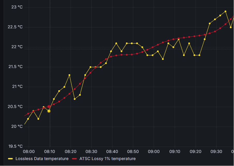
Image 1: ATSC data for temperature
How does ATSC work?
ATSC looks at the actual time series, in whole or in parts, to find how to better calculate a function that fits the existing data. For that, a quick statistical analysis is done, but if the results are inconclusive a sample is compressed with all the functions and the best function is selected.
By default, ATSC will segment the data—this guarantees better local fitting, more and smaller computations, and less memory usage. It also ensures that decompression targets a specific block instead of the whole file.
In each fitting frame, ATSC will create a function from a pre-defined set and calculate the parametrization of said function.
ATSC currently uses one (per frame) of those following functions:
- FFT (Fast Fourier Transforms)
- Constant
- Interpolation – Catmull-Rom
- Interpolation – Inverse Distance Weight
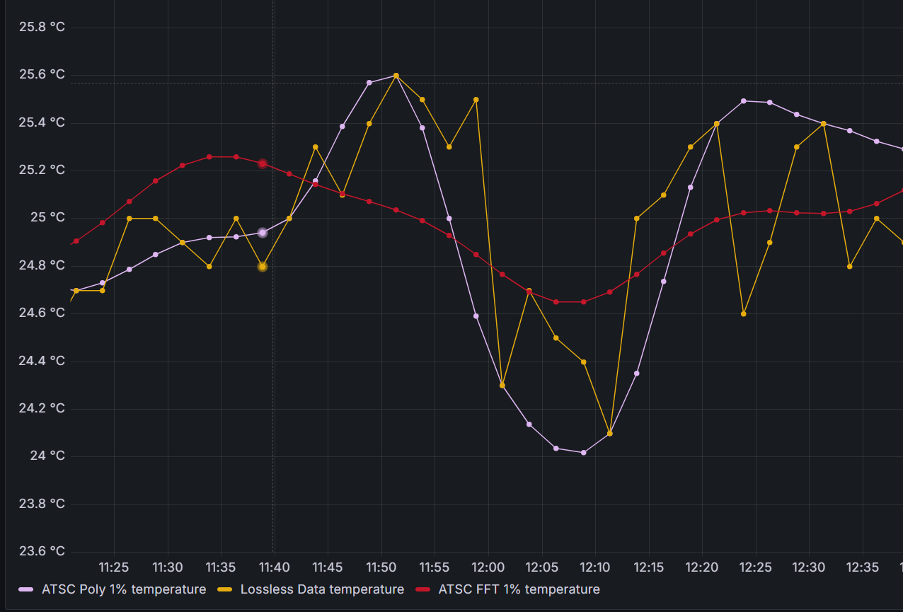
Image 2: Polynomial fitting vs. Fast-Fourier Transform fitting
These methods allow ATSC to compress data with a fitting error within 1% (configurable!) of the original time-series.
For a more detailed insight into ATSC internals and operations check our paper!
Use cases for ATSC and results
ATSC draws inspiration from established compression and signal analysis techniques, achieving compression ratios ranging from 46x to 880x with a fitting error within 1% of the original time-series. In some cases, ATSC can produce highly compressed data without losing any meaningful information, making it a versatile tool for various applications (please see use cases below).
Some results from our internal tests comparing to LZ4 and normal Prometheus compression yielded the following results:
| Method | Compressed size (bytes) | Compression Ratio |
| Prometheus | 454,778,552 | 1.33 |
| LZ4 | 141,347,821 | 4.29 |
| ATSC | 14,276,544 | 42.47 |
Another characteristic is the trade-off between fast compression speed vs. slower compression speed. Compression is about 30x slower than decompression. It is expected that time-series are compressed once but decompressed several times.

Image 3: A better fitting (purple) vs. a loose fitting (red). Purple takes twice as much space.
ATSC is versatile and can be applied in various scenarios where space reduction is prioritized over absolute precision. Some examples include:
- Rolled-over time series: ATSC can offer significant space savings without meaningful loss in precision, such as metrics data that are rolled over and stored for long term. ATSC provides the same or more space savings but with minimal information loss.
- Under-sampled time series: Increase sample rates without losing space. Systems that have very low sampling rates (30 seconds or more) and as such, it is very difficult to identify actual events. ATSC provides the space savings and keeps the information about the events.
- Long, slow-moving data series: Ideal for patterns that are easy to fit, such as weather data.
- Human visualization: Data meant for human analysis, with minimal impact on accuracy, such as historic views into system metrics (CPU, Memory, Disk, etc.)

Image 4: ATSC data (green) with an 88x compression vs. the original data (yellow)
Using ATSC
ATSC is written in Rust as and is available in GitHub. You can build and run yourself following these instructions.

Future work
Currently, we are planning to evolve ATSC in two ways (check our open issues):
- Adding features to the core compressor
focused on
these functionalities:
- Frame expansion for appending new data to existing frames
- Dynamic function loading to add more functions without altering the codebase
- Global and per-frame error storage
- Improved error encoding
- Integrations with
additional
technologies (e.g.
databases):
- We are currently looking into integrating ASTC with ClickHouse® and Apache Cassandra®
CREATE TABLE sensors_poly (
    sensor_id UInt16,
    location UInt32,
    timestamp DateTime,
    pressure Float64
CODEC(ATSC('Polynomial', 1)),
    temperature Float64
CODEC(ATSC('Polynomial', 1)),
)
ENGINE = MergeTree
ORDER BY (sensor_id, location,
timestamp);
Image 5: Currently testing ClickHouse integration
Sound interesting? Try it out and let us know what you think.
ATSC represents a significant advancement in time-series data compression, offering high compression ratios with a configurable accuracy loss. Whether for long-term storage or efficient data visualization, ATSC is a powerful open source tool for managing large volumes of time-series data.
But don’t just take our word for it—download and run it!
Check our documentation for any information you need and submit ideas for improvements or issues you find using GitHub issues. We also have easy first issues tagged if you’d like to contribute to the project.
Want to integrate this with another tool? You can build and run our demo integration with ClickHouse.
The post Innovative data compression for time series: An open source solution appeared first on Instaclustr.
New cassandra_latest.yaml configuration for a top performant Apache Cassandra®
Welcome to our deep dive into the latest advancements in Apache Cassandra® 5.0, specifically focusing on the cassandra_latest.yaml configuration that is available for new Cassandra 5.0 clusters.
This blog post will walk you through the motivation behind these changes, how to use the new configuration, and the benefits it brings to your Cassandra clusters.
Motivation
The primary motivation for introducing cassandra_latest.yaml is to bridge the gap between maintaining backward compatibility and leveraging the latest features and performance improvements. The yaml addresses the following varying needs for new Cassandra 5.0 clusters:
- Cassandra Developers: who want to push new features but face challenges due to backward compatibility constraints.
- Operators: who prefer stability and minimal disruption during upgrades.
- Evangelists and New Users: who seek the latest features and performance enhancements without worrying about compatibility.
Using cassandra_latest.yaml
Using cassandra_latest.yaml is straightforward. It involves copying the cassandra_latest.yaml content to your cassandra.yaml or pointing the cassandra.config JVM property to the cassandra_latest.yaml file.
This configuration is designed for new Cassandra 5.0 clusters (or those evaluating Cassandra), ensuring they get the most out of the latest features in Cassandra 5.0 and performance improvements.
Key changes and features
Key Cache Size
- Old: Evaluated as a minimum from 5% of the heap or 100MB
- Latest: Explicitly set to 0
Impact: Setting the key cache size to 0 in the latest configuration avoids performance degradation with the new SSTable format. This change is particularly beneficial for clusters using the new SSTable format, which doesn’t require key caching in the same way as the old format. Key caching was used to reduce the time it takes to find a specific key in Cassandra storage.
Commit Log Disk Access Mode
- Old: Set to legacy
- Latest: Set to auto
Impact: The auto setting optimizes the commit log disk access mode based on the available disks, potentially improving write performance. It can automatically choose the best mode (e.g., direct I/O) depending on the hardware and workload, leading to better performance without manual tuning.
Memtable Implementation
- Old: Skiplist-based
- Latest: Trie-based
Impact: The trie-based memtable implementation reduces garbage collection overhead and improves throughput by moving more metadata off-heap. This change can lead to more efficient memory usage and higher write performance, especially under heavy load.
create table … with memtable = {'class': 'TrieMemtable', … }
Memtable Allocation Type
- Old: Heap buffers
- Latest: Off-heap objects
Impact: Using off-heap objects for memtable allocation reduces the pressure on the Java heap, which can improve garbage collection performance and overall system stability. This is particularly beneficial for large datasets and high-throughput environments.
Trickle Fsync
- Old: False
- Latest: True
Impact: Enabling trickle fsync improves performance on SSDs by periodically flushing dirty buffers to disk, which helps avoid sudden large I/O operations that can impact read latencies. This setting is particularly useful for maintaining consistent performance in write-heavy workloads.
SSTable Format
- Old: big
- Latest: bti (trie-indexed structure)
Impact: The new BTI format is designed to improve read and write performance by using a trie-based indexing structure. This can lead to faster data access and more efficient storage management, especially for large datasets.
sstable:
  selected_format: bti
  default_compression: zstd
  compression:
    zstd:
      enabled: true
      chunk_length: 16KiB
      max_compressed_length: 16KiB
Default Compaction Strategy
- Old: STCS (Size-Tiered Compaction Strategy)
- Latest: Unified Compaction Strategy
Impact: The Unified Compaction Strategy (UCS) is more efficient and can handle a wider variety of workloads compared to STCS. UCS can reduce write amplification and improve read performance by better managing the distribution of data across SSTables.
default_compaction:
  class_name: UnifiedCompactionStrategy
  parameters:
    scaling_parameters: T4
    max_sstables_to_compact: 64
    target_sstable_size: 1GiB
    sstable_growth: 0.3333333333333333
    min_sstable_size: 100MiB
Concurrent Compactors
- Old: Defaults to the smaller of the number of disks and cores
- Latest: Explicitly set to 8
Impact: Setting the number of concurrent compactors to 8 ensures that multiple compaction operations can run simultaneously, helping to maintain read performance during heavy write operations. This is particularly beneficial for SSD-backed storage where parallel I/O operations are more efficient.
Default Secondary Index
- Old: legacy_local_table
- Latest: sai
Impact: SAI is a new index implementation that builds on the advancements made with SSTable Storage Attached Secondary Index (SASI). Provide a solution that enables users to index multiple columns on the same table without suffering scaling problems, especially at write time.
Stream Entire SSTables
- Old: implicity set to True
- Latest: explicity set to True
Impact: When enabled, it permits Cassandra to zero-copy stream entire eligible, SSTables between nodes, including every component. This speeds up the network transfer significantly subject to throttling specified by
entire_sstable_stream_throughput_outbound
and
entire_sstable_inter_dc_stream_throughput_outbound
for inter-DC transfers.
UUID SSTable Identifiers
- Old: False
- Latest: True
Impact: Enabling UUID-based SSTable identifiers ensures that each SSTable has a unique name, simplifying backup and restore operations. This change reduces the risk of name collisions and makes it easier to manage SSTables in distributed environments.
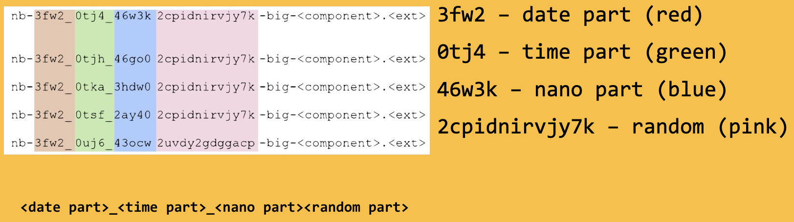
Storage Compatibility Mode
- Old: Cassandra 4
- Latest: None
Impact: Setting the storage compatibility mode to none enables all new features by default, allowing users to take full advantage of the latest improvements, such as the new sstable format, in Cassandra. This setting is ideal for new clusters or those that do not need to maintain backward compatibility with older versions.
Testing and validation
The cassandra_latest.yaml configuration has undergone rigorous testing to ensure it works seamlessly. Currently, the Cassandra project CI pipeline tests both the standard (cassandra.yaml) and latest (cassandra_latest.yaml) configurations, ensuring compatibility and performance. This includes unit tests, distributed tests, and DTests.
Future improvements
Future improvements may include enforcing password strength policies and other security enhancements. The community is encouraged to suggest features that could be enabled by default in cassandra_latest.yaml.
Conclusion
The cassandra_latest.yaml configuration for new Cassandra 5.0 clusters is a significant step forward in making Cassandra more performant and feature-rich while maintaining the stability and reliability that users expect. Whether you are a developer, an operator professional, or an evangelist/end user, cassandra_latest.yaml offers something valuable for everyone.
Try it out
Ready to experience the incredible power of the cassandra_latest.yaml configuration on Apache Cassandra 5.0? Spin up your first cluster with a free trial on the Instaclustr Managed Platform and get started today with Cassandra 5.0!
The post New cassandra_latest.yaml configuration for a top performant Apache Cassandra® appeared first on Instaclustr.
Cassandra 5 Released! What's New and How to Try it
Apache Cassandra 5.0 has officially landed! This highly anticipated release brings a range of new features and performance improvements to one of the most popular NoSQL databases in the world. Having recently hosted a webinar covering the major features of Cassandra 5.0, I’m excited to give a brief overview of the key updates and show you how to easily get hands-on with the latest release using easy-cass-lab.
You can grab the latest release on the Cassandra download page.
Instaclustr for Apache Cassandra® 5.0 Now Generally Available
NetApp is excited to announce the general availability (GA) of Apache Cassandra® 5.0 on the Instaclustr Platform. This follows the release of the public preview in March.
NetApp was the first managed service provider to release the beta version, and now the Generally Available version, allowing the deployment of Cassandra 5.0 across the major cloud providers: AWS, Azure, and GCP, and on–premises.
Apache Cassandra has been a leader in NoSQL databases since its inception and is known for its high availability, reliability, and scalability. The latest version brings many new features and enhancements, with a special focus on building data-driven applications through artificial intelligence and machine learning capabilities.
Cassandra 5.0 will help you optimize performance, lower costs, and get started on the next generation of distributed computing by:
- Helping you build AI/ML-based applications through Vector Search
- Bringing efficiencies to your applications through new and enhanced indexing and processing capabilities
- Improving flexibility and security
With the GA release, you can use Cassandra 5.0 for your production workloads, which are covered by NetApp’s industry–leading SLAs. NetApp has conducted performance benchmarking and extensive testing while removing the limitations that were present in the preview release to offer a more reliable and stable version. Our GA offering is suitable for all workload types as it contains the most up-to-date range of features, bug fixes, and security patches.
Support for continuous backups and private network add–ons is available. Currently, Debezium is not yet compatible with Cassandra 5.0. NetApp will work with the Debezium community to add support for Debezium on Cassandra 5.0 and it will be available on the Instaclustr Platform as soon as it is supported.
Some of the key new features in Cassandra 5.0 include:
- Storage-Attached Indexes (SAI): A highly scalable, globally distributed index for Cassandra databases. With SAI, column-level indexes can be added, leading to unparalleled I/O throughput for searches across different data types, including vectors. SAI also enables lightning-fast data retrieval through zero-copy streaming of indices, resulting in unprecedented efficiency.
- Vector Search: This is a powerful technique for searching relevant content or discovering connections by comparing similarities in large document collections and is particularly useful for AI applications. It uses storage-attached indexing and dense indexing techniques to enhance data exploration and analysis.
- Unified Compaction Strategy: This strategy unifies compaction approaches, including leveled, tiered, and time-windowed strategies. It leads to a major reduction in SSTable sizes. Smaller SSTables mean better read and write performance, reduced storage requirements, and improved overall efficiency.
- Numerous stability and testing improvements: You can read all about these changes here.
All these new features are available out-of-the-box in Cassandra 5.0 and do not incur additional costs.
Our Development team has worked diligently to bring you a stable release of Cassandra 5.0. Substantial preparatory work was done to ensure you have a seamless experience with Cassandra 5.0 on the Instaclustr Platform. This includes updating the Cassandra YAML and Java environment and enhancing the monitoring capabilities of the platform to support new data types.
We also conducted extensive performance testing and benchmarked version 5.0 with the existing stable Apache Cassandra 4.1.5 version. We will be publishing our benchmarking results shortly; the highlight so far is that Cassandra 5.0 improves responsiveness by reducing latencies by up to 30% during peak load times.
Through our dedicated Apache Cassandra committer, NetApp has contributed to the development of Cassandra 5.0 by enhancing the documentation for new features like Vector Search (Cassandra-19030), enabling Materialized Views (MV) with only partition keys (Cassandra-13857), fixing numerous bugs, and contributing to the improvements for the unified compaction strategy feature, among many other things.
Lifecycle Policy Updates
As previously communicated, the project will no longer maintain Apache Cassandra 3.0 and 3.11 versions (full details of the announcement can be found on the Apache Cassandra website).
To help you transition smoothly, NetApp will provide extended support for these versions for an additional 12 months. During this period, we will backport any critical bug fixes, including security patches, to ensure the continued security and stability of your clusters.
Cassandra 3.0 and 3.11 versions will reach end-of-life on the Instaclustr Managed Platform within the next 12 months. We will work with you to plan and upgrade your clusters during this period.
Additionally, the Cassandra 5.0 beta version and the Cassandra 5.0 RC2 version, which were released as part of the public preview, are now end-of-life You can check the lifecycle status of different Cassandra application versions here.
You can read more about our lifecycle policies on our website.
Getting Started
Upgrading to Cassandra 5.0 will allow you to stay current and start taking advantage of its benefits. The Instaclustr by NetApp Support team is ready to help customers upgrade clusters to the latest version.
- Wondering if it’s possible to upgrade your workloads from Cassandra 3.x to Cassandra 5.0? Find the answer to this and other similar questions in this detailed blog.
- Click here to read about Storage Attached Indexes in Apache Cassandra 5.0.
- Learn about 4 new Apache Cassandra 5.0 features to be excited about.
- Click here to learn what you need to know about Apache Cassandra 5.0.
Why Choose Apache Cassandra on the Instaclustr Managed Platform?
NetApp strives to deliver the best of supported applications. Whether it’s the latest and newest application versions available on the platform or additional platform enhancements, we ensure a high quality through thorough testing before entering General Availability.
NetApp customers have the advantage of accessing the latest versions—not just the major version releases but also minor version releases—so that they can benefit from any new features and are protected from any vulnerabilities.
Don’t have an Instaclustr account yet? Sign up for a trial or reach out to our Sales team and start exploring Cassandra 5.0.
With more than 375 million node hours of management experience, Instaclustr offers unparalleled expertise. Visit our website to learn more about the Instaclustr Managed Platform for Apache Cassandra.
If you would like to upgrade your Apache Cassandra version or have any issues or questions about provisioning your cluster, please contact Instaclustr Support at any time.
The post Instaclustr for Apache Cassandra® 5.0 Now Generally Available appeared first on Instaclustr.
easy-cass-lab v5 released
I’ve got some fun news to start the week off for users of easy-cass-lab: I’ve just released version 5. There are a number of nice improvements and bug fixes in here that should make it more enjoyable, more useful, and lay groundwork for some future enhancements.
- When the cluster starts, we wait for the storage service to
reach NORMAL state, then move to the next node. This is in contrast
to the previous behavior where we waited for 2 minutes after
starting a node. This queries JMX directly using Swiss Java Knife
and is more reliable than the 2-minute method. Please see
packer/bin-cassandra/wait-for-up-normalto read through the implementation. - Trunk now works correctly. Unfortunately, AxonOps doesn’t support trunk (5.1) yet, and using the agent was causing a startup error. You can test trunk out, but for now the AxonOps integration is disabled.
- Added a new repl mode. This saves keystrokes and provides some
auto-complete functionality and keeps SSH connections open. If
you’re going to do a lot of work with ECL this will help you be a
little more efficient. You can try this out with
ecl
repl
. - Power user feature: Initial support for profiles in AWS regions
other than
us-west-2. We only provide AMIs forus-west-2, but you can now set up a profile in an alternate region, and build the required AMIs usingeasy-cass-lab build-image. This feature is still under development and requires using aneasy-cass-labbuild from source. Credit to Jordan West for contributing this work. - Power user feature: Support for multiple profiles. Setting the
EASY_CASS_LAB_PROFILEenvironment variable allows you to configure alternate profiles. This is handy if you want to use multiple regions or have multiple organizations. - The project now uses Kotlin instead of Groovy for Gradle configuration.
- Updated Gradle to 8.9.
- When using the list command, don’t show the alias “current”.
- Project cleanup, remove old unused pssh, cassandra build, and async profiler subprojects.
The release has been released to the project’s GitHub page and to homebrew. The project is largely driven by my own consulting needs and for my training. If you’re looking to have some features prioritized please reach out, and we can discuss a consulting engagement.
easy-cass-lab updated with Cassandra 5.0 RC-1 Support
I’m excited to announce that the latest version of easy-cass-lab now supports Cassandra 5.0 RC-1, which was just made available last week! This update marks a significant milestone, providing users with the ability to test and experiment with the newest Cassandra 5.0 features in a simplified manner. This post will walk you through how to set up a cluster, SSH in, and run your first stress test.
For those new to easy-cass-lab, it’s a tool designed to streamline the setup and management of Cassandra clusters in AWS, making it accessible for both new and experienced users. Whether you’re running tests, developing new features, or just exploring Cassandra, easy-cass-lab is your go-to tool.
easy-cass-lab now available in Homebrew
I’m happy to share some exciting news for all Cassandra enthusiasts! My open source project, easy-cass-lab, is now installable via a homebrew tap. This powerful tool is designed to make testing any major version of Cassandra (or even builds that haven’t been released yet) a breeze, using AWS. A big thank-you to Jordan West who took the time to make this happen!
What is easy-cass-lab?
easy-cass-lab is a versatile testing tool for Apache Cassandra. Whether you’re dealing with the latest stable releases or experimenting with unreleased builds, easy-cass-lab provides a seamless way to test and validate your applications. With easy-cass-lab, you can ensure compatibility and performance across different Cassandra versions, making it an essential tool for developers and system administrators. easy-cass-lab is used extensively for my consulting engagements, my training program, and to evaluate performance patches destined for open source Cassandra. Here are a few examples: