High-Throughput Graph Abstraction at Netflix: Part I
By Oleksii Tkachuk, Kartik Sathyanarayanan, Rajiv Shringi
Introduction
Netflix has a diverse range of graph use cases, each serving specific business needs with unique functionality and performance requirements. These use cases fall into two broad categories:
- OLAP: These use cases typically involve open-ended and algorithmic exploration of large graph datasets. They often utilize industry-standard models and languages such as RDF with SPARQL, Property Graphs with Gremlin or openCypher, and even SQL. The primary focus in these situations is in-depth analysis, rather than achieving high throughput and low latency.
- OLTP: These use cases require extremely high throughput — up to millions of operations per second — while delivering traversal results within milliseconds. Achieving such a level of performance often requires making trade-offs, which can include accepting eventual consistency or restricting query complexity. For example, the service can demand a specified starting point for traversals and enforce a maximum traversal depth. Such use cases are often directly tied to streaming or user experiences and demand high global availability.
Netflix’s Graph Abstraction was designed specifically for this second category of use cases. As of this writing, the abstraction is handling close to 10 million operations per second across 650 TB of graph datasets with low latency and cost efficiency.
This post is the first in a multi-part series that explores the Graph Abstraction architecture in depth. We’ll cover how the abstraction indexes data for real-time and historical views, manages strongly typed graphs, performs efficient traversals, and integrates with the Netflix Big Data ecosystem.
Usage at Netflix
From a business standpoint, the primary driver for developing the Graph Abstraction was internal demand for supporting several key use cases:
- Real-Time Distributed Graph (RDG): A graph capturing dynamic relationships across entities and interactions throughout the Netflix ecosystem. You can learn more about the initial RDG implementation in this insightful blog post. This functionality has since been integrated into the Graph Abstraction.
- Social Graph: A graph of social connections within Netflix Gaming, designed to boost user engagement.
- Service Topology: A graph of all internal Netflix services, used for real-time and historical analysis to improve root cause analysis during incidents.
Let’s examine the overall architecture of the Graph Abstraction and how it integrates with the Netflix Online Datastore ecosystem.
Architecture
Instead of building the persistence and caching layers from scratch, we chose to build taller on top of existing Netflix data abstractions.

The Key-Value (KV) Abstraction stores the latest view of nodes and edges, serving as the real-time index for all queries. Optionally, users can plug-in the TimeSeries (TS) Abstraction if they are interested in a historical view of how the graph evolves over time. Additionally, we use EVCache to achieve low-millisecond latencies and are actively experimenting with more specialized caching layers to further improve performance. Finally, the Graph Abstraction integrates with the Data Gateway Control Plane to manage graph schemas and automate the provisioning, deletion, and configuration of datasets in both KV and TS.
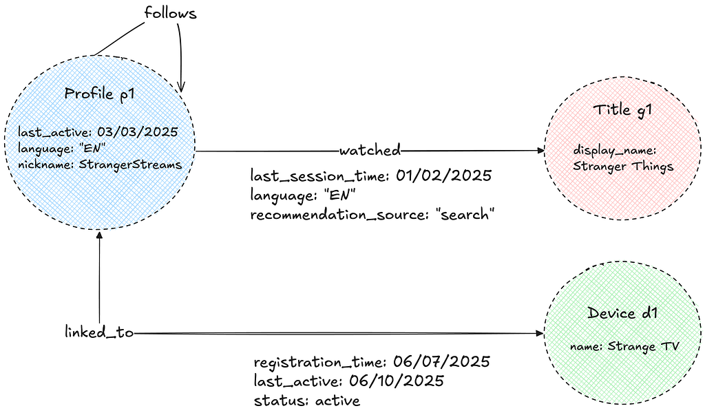
Property Graph Model
The Abstraction uses the Property Graph model to store its data. The graph consists of nodes and edges of various types, each with associated properties. These properties are strongly typed to enable efficient filtering and ensure consistent data exports. For semantic reasons, edges can be either unidirectional or bidirectional.
Namespaces
The Abstraction separates data into isolated units called “namespaces.” Each namespace is associated with a physical storage layer, as configured in the Data Gateway Control Plane, and can be deployed on either dedicated or shared hardware. The optimal, most cost-effective hardware configuration is determined by our provisioning automation, based on user-provided requirements such as throughput, latency, dataset size, and workload criticality. For more details on this topic, see this talk given by our stunning colleague Joey Lynch at AWS re:Invent.
Graph Schema
Each namespace is further associated with an explicit graph schema configured in the Control Plane. The graph schema defines node and edge types, allowed properties, permitted relationships, and directions.
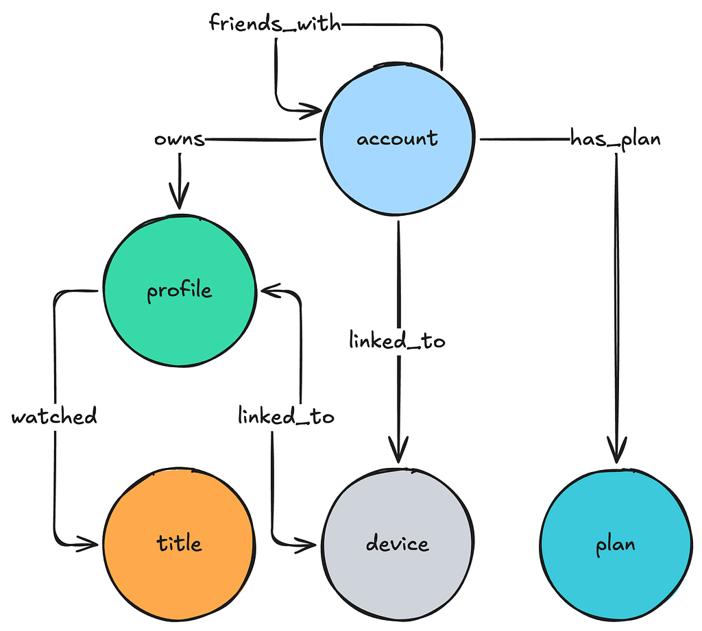
The Graph schema is implemented as a collection of edge mappings that describe the nature of the relationship between given node types.
{
  "edgeConfig": {
    "edgeMappings": [
      {
        "edgeMappingKey": {
          "fromNodeType": "account",
          "edgeType": "owns",
          "toNodeType": "profile"
        },
        "directionType": "UNIDIRECTIONAL"
      },
      {
        "edgeMappingKey": {
          "fromNodeType": "profile",
          "edgeType": "linked_to",
          "toNodeType": "device"
        },
        "directionType": "BIDIRECTIONAL"
      }
    ]
  }
}
Edge mappings are further extended with specification of property schema that consists of allowed property names and their type specification:
{
   "edgeMappingKey":{
      "fromNodeType":"profile",
      "edgeType":"linked_to",
      "toNodeType":"device"
   },
   "propertySchema":{
      "propertyMappings":[
         { "propertyKey":"registration_time", "propertyValueType":"TIMESTAMP" },
         { "propertyKey":"status", "propertyValueType":"STRING" }
      ]
   }
}
The Abstraction servers load this schema on startup and build an in-memory metadata graph of possible relationships, enabling several key optimizations:
- Data Quality: The Abstraction rejects non-conforming nodes, edges, and properties during writes, ensuring high data quality and consistent exports.
- Query Planning: The Abstraction uses the schema to quickly construct the possible traversal paths the service should take to answer a given user query.
- Deduplication of Traversed Edges: For bidirectional traversals on edges between the same node type, the schema helps avoid redundant processing by deduplicating traversed paths.
- Eliminating Traversal paths: For a given user query, the Abstraction removes traversal paths associated with impossible relationships, as well as those where filters or property types are incompatible.
Further, the Abstraction servers periodically poll the schema from the Data Gateway Control Plane in order to keep it updated with user changes. Looking ahead, we plan to leverage the graph schema for additional improvements, such as:
- Minimizing Query Fanout: By using edge cardinality within edge mappings, we aim to select the most efficient traversal paths and minimize query fanout.
- Improved Developer Experience: The schema will support generating a type-safe data access layer and enhance the Gremlin-like API with schema awareness.
Next, let’s look at how this data is organized in a real-time index within the KV Abstraction.
Real-Time Index: Key-Value Storage
Before we discuss how the data is organized into graph indexes, let’s discuss how KV organizes data within namespaces and provides idempotency guarantees:
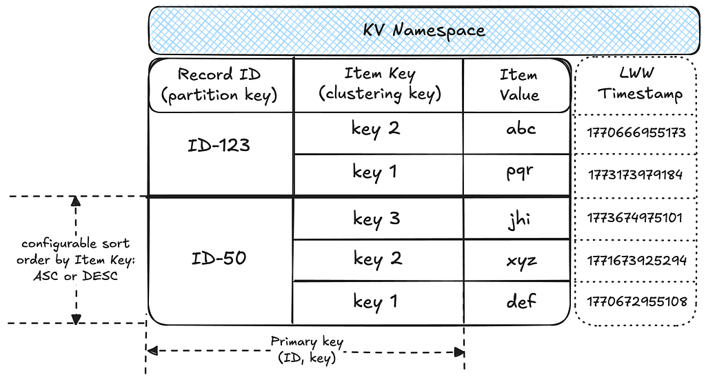
- Data partitioning: A namespace is associated with a table in the underlying storage layer. Within the table, data is partitioned into records by unique IDs, with each record holding multiple sorted items as key-value pairs. This structure effectively makes each namespace a map of sorted maps, providing flexibility for diverse access patterns.
- Idempotency: Writes to a given ID and key are idempotent, enabling request hedging and safe retries. The idempotency token contains a timestamp, which KV uses to enforce Last-Write-Wins (LWW) semantics at the storage layer.
We use the KV as the underlying storage for all real-time graph indices on nodes and edges. For more on Netflix’s Key-Value Abstraction, see this excellent post published by our KeyValue team.
Node Storage
The two-tiered partitioning strategy works well for node storage. Each node type is isolated within its own KV namespace, which stores all the properties for nodes of that type.
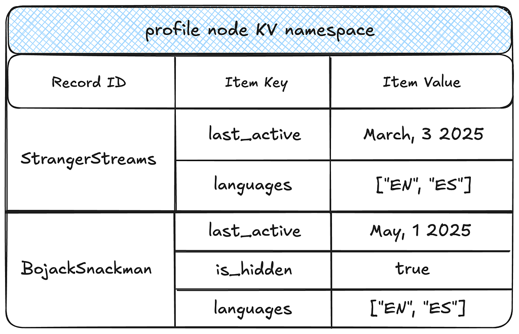
This storage format enables several efficient access patterns for nodes:
- Efficient reads: A given node and all its properties are fetched in a single partition lookup, achieving single-digit millisecond latency.
- Property selection pushdown: Target property keys are pushed down to the KV layer, reducing the amount of data fetched and further decreasing latencies and network overhead.
- Property filtering pushdown: Property keys and values can be efficiently filtered at the KV layer.
- Efficient exports: This model supports highly parallelized node exports by node type.
Edge Storage
Links and Property Index
Edges utilize two distinct types of indexes: one exclusively for the edge connections (links), and one for edge properties.
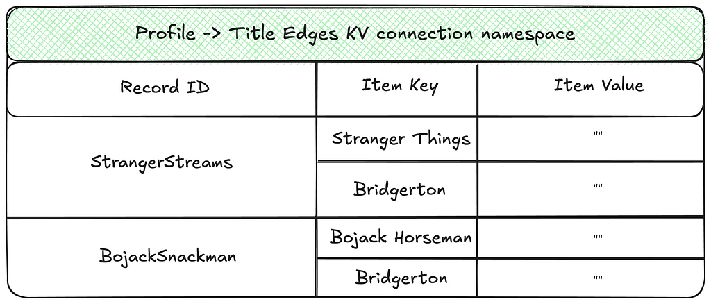
The Edge links are arranged as an adjacency list mapping source nodes to their connected neighbors.
The Edge Property index stores information about properties of every edge.

Separating edge links from their properties brings several benefits, but also introduces a key trade-off:
Benefits:
- Efficient property upserts: Allows individual properties to be upserted over time without needing to read the entire property set for an edge.
- Wide row prevention: Decoupling edge links from their properties prevents large partitions in databases like Cassandra, enabling efficient storage and low-latency reads — even for edges with millions of connections.
Trade-off:
- Non-atomic writes: Storing edges across multiple namespaces means that writes across these namespaces are not atomic. We’ll discuss how this is addressed in the Consistency Enforcement section.
Forward and Reverse Indexes
Additionally, edge indexes are separated into forward and reverse indexes to support traversals in either direction. The illustration below shows an example of the reverse index counterpart for the links namespace shown above.

To ensure consistent record identifiers when updating edge properties in either direction, the Abstraction lexicographically sorts and concatenates the source and destination node IDs to create a direction-agnostic identifier for property storage. This ensures that properties can be accessed or mutated in a single database call regardless of the direction specified in the request.

This storage format enables several efficient access patterns:
- Point Reads: Given an edge id, all properties can be fetched in a single partition lookup on the properties index.
- Range Reads: Given a source node, a range read on a partition in the links index can efficiently return all edges. Depending on the desired direction, the Abstraction can target the forward or reverse index.
- Property Filtering: Properties are fetched only for the links that match the record or page limit criteria, minimizing the data exchanged over the network.
- Sort Orders: By default, edge links are sorted lexicographically by their target node. To support fetching the latest connections, the Abstraction retrieves target edge links in memory, sorts them by their last-write time, and returns the results. In order to ensure optimal performance without exerting too much memory pressure, we aim to limit the number of edges per source node within the system.
Next, let’s explore the caching strategies used by the Abstraction.
Caching Strategies in Graph Abstraction
Although the Graph Abstraction already provides efficient reads and writes to durable storage, caching remains critical for the stability and performance of any graph datastore for two key reasons:
- Write amplification: A single write on the fronting service can result in multiple writes to the backing durable storage due to the use of multiple indexes. Whenever possible, it’s best to avoid unnecessary writes — for example, by not writing an edge link that already exists.
- Read amplification: A single traversal request on the fronting service may translate into thousands of fetch operations on the backend, especially for highly interconnected graphs.
To address these challenges, the Graph Abstraction employs two distinct caching strategies.
Write-aside Caching of Edge Links
An edge link contains no additional information beyond the link itself and its last-write timestamp. To reduce write amplification on durable storage, we cache edge links for short durations, helping to avoid writing a link that already exists. This mechanism is balanced with configurable TTL windows, cache invalidation on deletes, and lease acquisitions with exponential backoff. These strategies provide the necessary consistency guarantees while still allowing the last-write timestamp to be refreshed according to the predefined staleness.

Read-aside Caching of Properties
To reduce read amplification on the durable store, the Graph Abstraction leverages KV’s integration with EVCache. Multiple KV namespaces can share the same caching clusters for cost efficiency. The Abstraction first fetches data from durable storage, while subsequent reads are served from the cache. Caching is applied at both the record and item levels, benefiting all graph objects.
Graph Abstraction employs two invalidation strategies, selected based on write throughput and consistency requirements:
- Invalidation on write: Both record and item caches are invalidated with every write, ensuring consistency across regions. This strategy is ideal for graphs that change infrequently and cannot tolerate data staleness, but comes with the tradeoff of pushing a higher throughput on the cache.
- TTL-driven invalidation: Cache entries are invalidated only when their TTL expires. This approach works best for frequently modified objects that can tolerate some staleness.
Work In Progress: Write-Through Caching
We are also developing a write-through caching strategy designed to store most of the data required by the Abstraction during traversals. This caching mechanism can organize indexes by different sort orders (e.g., sorting data by last-write timestamp), at the cost of increased memory consumption. Stay tuned for more details on this approach.
Next, let’s examine the consistency guarantees in Graph Abstraction and how they are enforced for both reads and writes.
Consistency Enforcement
Enforcing data consistency in Graph Abstraction poses several challenges. The connected nature of the data, low-latency API requirements, and the need to handle intermittent failures have led to design choices that enforce strict eventual consistency across multiple regions.
Entropy Repair
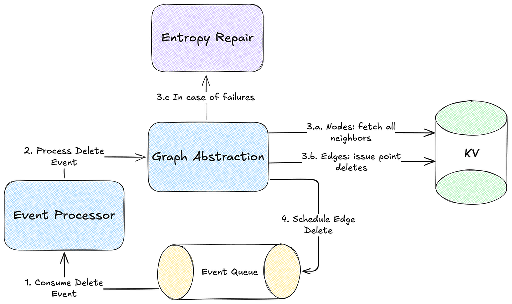
Each write in the Abstraction persists data for both inward and outward indices in parallel to support high throughput. Further, each write happens on multiple KV namespaces. To prevent inconsistencies or lasting entropy from failures in any operation, the Abstraction uses a robust retry mechanism using Kafka:

Node Deletions
Deleting nodes in a highly connected graph is more complex than simply removing a KV record as each node may have thousands of connected edges that must be handled to maintain graph integrity. Further, synchronously deleting all such connections would introduce unacceptable latency for the Abstraction callers.
The Abstraction employs an asynchronous deletion strategy to manage this issue. The consequence of this approach, however, is that the observed mutated state is only eventually consistent. Further, to ensure correctness of asynchronous deletes during concurrent updates, the Last-Write-Wins (LWW) conflict resolution mechanism is essential.
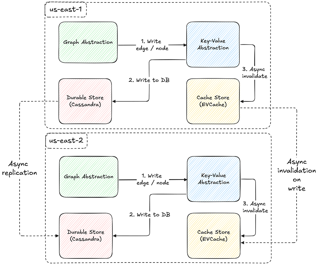
Global Replication
The consistency guarantees of Graph Abstraction are shaped by its multi-region availability. As illustrated in the diagram below, both the caching layer and durable storage replicate data asynchronously across regions, resulting in an eventually consistent system.
Now that we’ve covered storing the real-time graph index, let’s see how it enables graph traversals.
Graph Traversals
The Abstraction provides a custom gRPC traversal API, inspired by Gremlin, which enables exploration of the distributed graph by letting users chain traversals, apply filter criteria, sort results, limit results, and more.
Let’s explore a hypothetical scenario where the Abstraction is used to recommend shows to users on a shared device, by considering the duration of the most recent viewing session for each show across all profiles and accounts associated with that device:
TraversalRequest.newBuilder()
  .setNamespace("<graph-namespace>")
  .setTraversalQuery(
     TraversalQuery.newBuilder()
       // Given id of the 'device' node type.
       .setStartNode(node("device", "my-device-id"))
       .setTraversal(
          Traversal.newBuilder()
            // fetch the first 5 connections
            .setEdgeLimit(5)
            .setDirectionTraversal(
               DirectionTraversal.newBuilder()
                  // traverse in the IN direction
                  .setDirection(IN)
                  // minimize data exchange: only interested in certain properties
                  .addNodePropertiesSelections(propSelection("account", "created_at"))
                  .addNodePropertiesSelections(propSelection("profile", "last_active"))
                  .setDirectionFilter(
                     DirectionFilter.newBuilder()
                       // only interested in certain connected types
                       .setTypeMatchingStrategy(EXCLUDE_NON_TARGETED)
                       .addAllNodeFilters(typeFilters("account", "profile"))))
            // chain traversals to the intermediate result
            .addNextTraversals(
               Traversal.newBuilder()
                 .setOrder(LATEST)
                 // limit to 200 connections for the 2nd hop
                 .setEdgeLimit(200)
                 .setDirectionTraversal(
                    DirectionTraversal.newBuilder()
                      // now traverse in the OUT direction
                      .setDirection(OUT)
                      .addEdgePropertiesSelections(propSelection("watched", "view_time"))
                      .addEdgePropertiesSelections(propSelection("has_plan", "active"))
                      .setDirectionFilter(
                         DirectionFilter.newBuilder()
                           .setTypeMatchingStrategy(EXCLUDE_NON_TARGETED)
                           .addAllNodeFilters(typeFilters("title", "plan")))))))
  .build();
And let’s visualize the intended results set produced by the request above:

We’ll explore the design and implementation of traversal planning and execution, along with different traversal types, in the Part II of this blog series.
Now let’s look at the performance metrics of Graph Abstraction based on current production use cases.
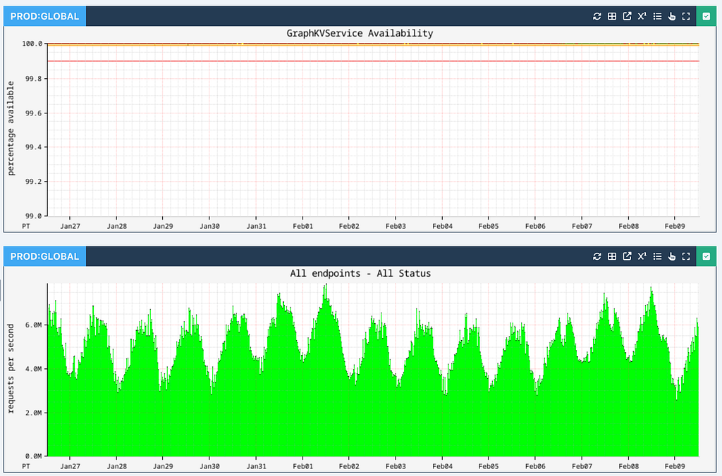
Real World Performance
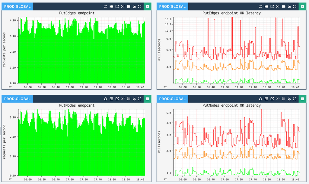
Across all applications at Netflix, Graph Abstraction ensures high availability while processing up to 10 million operations per second across all writes, individual edge / node reads and traversals at peak hours:
Edge and node persistence achieve single-digit millisecond latencies (p99 shown in red, p90 shown in orange, and p50 shown in green):
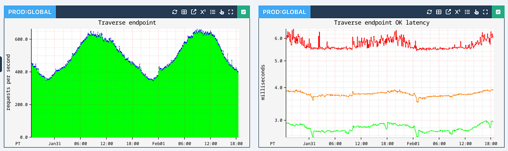
Traversal performance depends on the number of hops, the edge fanout at each stage, and associated filters and sort orders. We parallelize work as much as possible to reduce latencies. Typically 1-hop traversals are executed with single-digit millisecond latency:
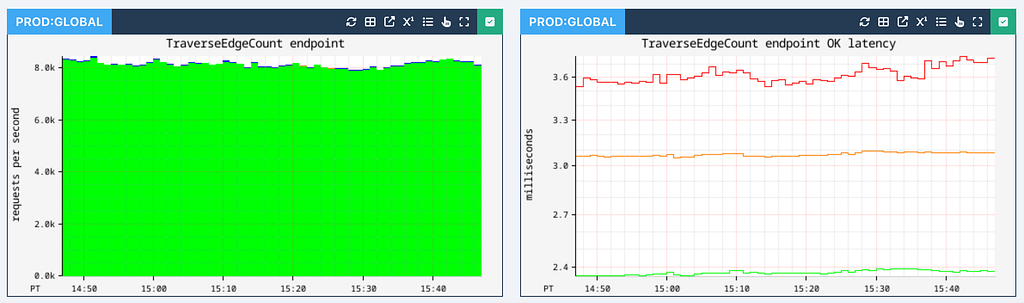
We also support a Count API that performs counting traversals at a very high rate with similar latencies, which we will cover in Part II of this series:
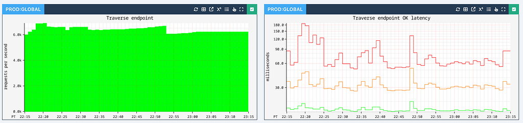
Currently, the RDG is powered by 2-hop traversals with a higher degree of fan-out. While these operations can reach upwards of 100 ms in latency, the 90th percentile (p90) latency remains under 50ms.
We track the average and max edge fanout at different depths to give us insights into the traversal performance for different graph datasets.


Asynchronous operations such as node deletions can be slightly latent, but typically perform with sub-second latency:
At the moment, we are storing close to 650 TB of data globally across all our graph datasets.

Conclusion
As Netflix scales further into new verticals such as live content, games, and ads, Graph Abstraction will remain crucial for uncovering and leveraging rich connections — while continuing to support a high throughput and availability at low latencies.
Stay tuned for Part II of this blog series, where we’ll explore the implementation of graph traversals, counting and constraint mechanisms.
In Part III, we’ll take a closer look at the temporal index implementation and its integration with the Time Series Abstraction.
Acknowledgments
Special thanks to our stunning colleagues who contributed to Graph Abstraction’s success: Kaidan Fullerton, Joey Lynch, Sudhesh Suresh, Vinay Chella, Sumanth Pasupuleti, Vidhya Arvind, Raj Ummadisetty, Jordan West, Chris Lohfink, Joe Lee, Jingxi Huang, Jessica Walton, Prudhviraj Karumanchi, Akashdeep Goel, Sriram Rangarajan, Chris Van Vlack, Christopher Gray, Luis Medina, Ajit Koti, Mohidul Abedin.
High-Throughput Graph Abstraction at Netflix: Part I was originally published in Netflix TechBlog on Medium, where people are continuing the conversation by highlighting and responding to this story.
ScyllaDB Customer Experience Spotlight: Tyler Denton
Welcome to the first installment of a new blog series introducing some of the experts you’re likely to encounter when you work with ScyllaDB. Tyler Denton is a Solutions Architect on the Customer Experience team here at ScyllaDB. He lives in Fort Myers Florida, USA. He’s been at ScyllaDB for about a year, Let’s get to know a little about Tyler… What do you do here at ScyllaDB I’m a Solutions Architect, which is sometimes known as a Sales Engineer or Solutions Engineer. I help customers or prospects review their architectures and find the best place for ScyllaDB to be deployed. Does it make sense, and what’s the most efficient, impactful way to use ScyllaDB in their product or solution? I’m also our field AI subject Subject Matter Expert, so I do a lot with our vector search, a lot with our feature store deployments, agent, state management…things like that. Please share a little about your path to ScyllaDB My first job ever was as a machinist’s mate operating nuclear reactors in the US Navy. That might seem like an odd place to start for somebody who works as a Solutions Architect…but what that taught me was systems. How does the failure of a main steam root valve affect the starboard steam generators? Understanding how complex systems interact and work together taught me a lot about architecture and how to build systems that can survive failure. I started writing software in about the sixth grade and continued doing that, and so I’ve worked at companies like AWS, Couchbase, Rockset (acquired by OpenAI), and that all kind of led me here — where I can focus heavily on bringing large, distributed systems into production and focusing on AI. Tell me about one of the most interesting projects you’ve worked on here One of the most interesting projects I’ve worked on here is an AdTech company that used every feature of our flagship product, ScyllaDB X Cloud. We got to see the major, nearly instantaneous scaling of ScyllaDB. If anybody’s ever used Cassandra or earlier versions of ScyllaDB, you know that wide-table databases can be very hard to scale and can take a long time. Here, we were able to go from 6 nodes to 60 nodes in about 15 minutes, and the throughput and performance we saw from that was absolutely incredible. Watching this develop in real time was very cool and very rewarding. What’s the most impressive ScyllaDB feat you’ve seen a team accomplish Right now, I’m working on bringing a deployment into production where we were displacing another technology. By moving from their existing data model to one supported in ScyllaDB using static maps, we saw a huge cost reduction and a huge performance improvement. They were able to support queries across very complicated data structures in sub-millisecond latency across their entire corpus of data, and they were able to do that because they migrated to ScyllaDB. What do you like to do when you’re not working or on-call When I’m not working my day job, I focus a lot on building my AI knowledge. I do a lot of speaking engagements, development work, and community outreach. And when I’m not doing that, I’m working on my boat. Every now and then I actually get to take it out, but anybody who owns a boat knows that most of the time is spent actually working on it. What’s your top tip for getting the most out of ScyllaDB Follow the instructions. RTFM. Don’t try to be unique. ScyllaDB is designed to solve very specific use cases, and it does that incredibly well. When you try to get creative and build a database within a database, or start doing things ScyllaDB wasn’t designed for, it gets painful really fast, and ScyllaDB will punish you. So just read the manual, follow the best practices, and you’ll have a great time.
ScyllaDB Elastic Scaling in Action [Demo]
Watch along to see how fast ScyllaDB X Cloud scales from 10K to 1M ops/sec and back down again – with single-digit millisecond latency ScyllaDB X Cloud is ScyllaDB’s fully-managed database-as-a-service. It’s a truly elastic database designed to support variable/unpredictable workloads with consistent low latency as well as low costs. We’ve previously blogged about how users can scale out and scale in almost instantly to match actual usage. For example, you can scale all the way from 100K OPS to 2M OPS in just minutes, with consistent single-digit millisecond P99 latency. This means you don’t need to overprovision for the worst-case scenario or suffer the lag traditionally associated with ramping up capacity in response to a sudden surge. In this post, I want to show you how it looks in action: increasing capacity 10X, as well as scaling it back, in minutes. Part 1: Scaling 10X Fast, with Single-Digit Millisecond P99 Latency This first video provides a quick look at how fast ScyllaDB XCloud scales out to increase capacity. It shows you how ScyllaDB’s new tablets architecture lets you scale a cluster to support 10x or more workload capacity in minutes (vs. the usual hours or days). Simulating a massive sales event, we scale a cluster from a moderate 100K ops/sec up to 1M. As we start, the cluster is currently managing a moderate load of 100K ops/sec across three small nodes. Knowing that a surge of 1M ops/sec is imminent, we use the built-in calculator to precisely size our needs. By simply entering the desired read and write throughput and selecting the schema complexity, the system automatically determines the necessary vCPU requirement. In this case, we add three larger nodes to our existing setup. Once the new scaling policy is saved, you can watch the scaling happen as the nodes join and tablets are automatically streamed and rebalanced in parallel. In this demo, the entire scale-out process, including data rebalancing, completed in roughly 23 minutes—all while the cluster remained under load. You’ll see that the new nodes immediately start sharing the responsibility of serving requests even before the rebalancing is fully finished. Finally, we simulate the 10x load jump to 1 million operations per second. You can see that even with mixed instance sizes, ScyllaDB perfectly balances the workload, with the larger nodes serving more requests as expected. Most importantly, despite this massive increase in traffic, the cluster maintains impressive performance. It achieves single-digit millisecond P99 latencies throughout the entire event. Part 2: Achieving Rapid Parallel Scale-Down After Peak Workload This next video demonstrates the process of scaling the ScyllaDB cluster back down to its original size following a simulated high-traffic sales event. You can see how the system handles a drop from 1M ops/sec down to its baseline load. After running at 1M ops/sec for about 20 minutes, our simulated sale event has concluded. That means our load is dropping back to its original 100K ops/sec. Once the load stabilizes and the monitoring overview panel confirms that we are back to 20K writes and 80K reads, we’re ready to scale the cluster back to its original size of 24 vCPUs. To do this, we simply update the scaling policy back to 24 vCPUs. That leaves us with the same three 2x large nodes we had before the simulated sale event started. As the scaling progress begins, we can watch the nodes leave the cluster in real-time. By viewing the monitoring dashboard’s detailed panel, we can see an animation of the tablets streaming from the larger 8x nodes back to the original nodes. Once that’s completed, the cluster is back to its original configuration of three nodes. The scale-down process took about 22 or 23 minutes, which is nearly identical to the time it took to scale up earlier (in the other video). While scaling out has always been fast with tablets, scaling back down used to be a sequential process. Now, starting with version ScyllaDB 2026.1.3, we can scale the cluster in parallel both out and back. That makes it possible to handle a massive workload spike and return to baseline capacity all within about an hour. ScyllaDB Cloud – Free TrialApache Cassandra Performance Tuning: What We Learned
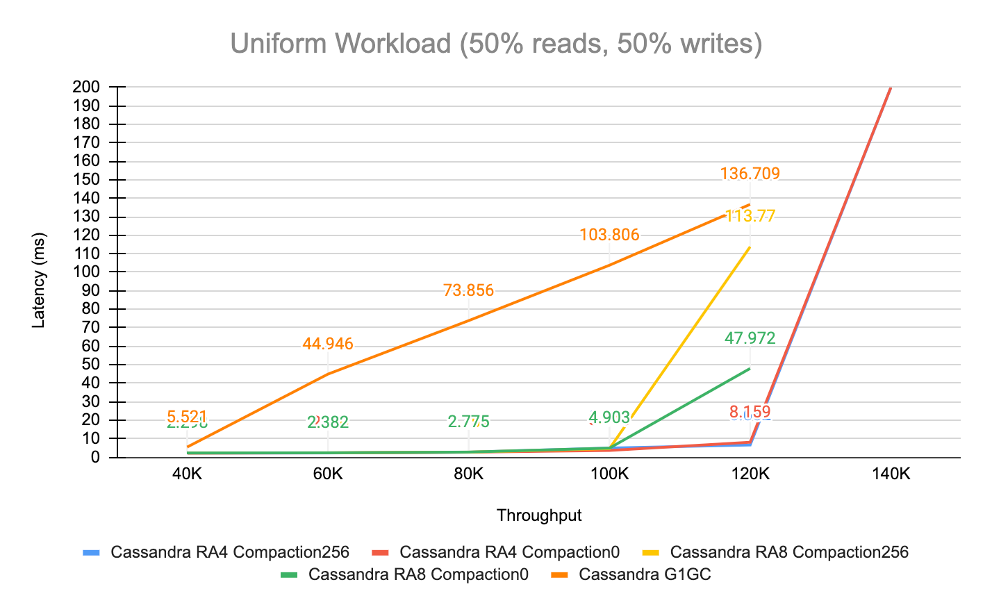
This blog post (tries to) consolidate what we’ve learned from years of tuning Apache Cassandra for performance Here at ScyllaDB, we often run internal and external performance comparisons. Internal testing helps ensure ScyllaDB’s performance advantage, track performance regressions, and maintain compatibility, including catching subtle API semantic-layer changes early. External comparisons are our way to aggregate the performance results for the general public every once in a while. Performance tuning can be a double-edged sword. Overlook one aspect, and you may end up under- or overestimating one’s performance numbers – and that may introduce deep ramifications down the road. While ScyllaDB and Cassandra both share a common API layer and feature set, both systems have fundamentally different architectures. This naturally adds to differences in how each system is tested and tuned. This blog post (tries to) consolidate what we’ve learned from years of tuning Apache Cassandra for performance. We spent a good amount of time hunting down the information we needed. Hopefully, the details described here help others improve their existing Cassandra cluster performance, as well as conduct more meaningful performance comparisons. Side-note: ScyllaDB shares how to reproduce our tests, including references on which settings and parameters we tuned. Check out our Cassandra 4 vs Cassandra 3.11 comparison, my recent talk on how ScyllaDB compares to Cassandra 5, and the comparison between Cassandra vNodes and ScyllaDB tablets as some concrete examples. Overview Perhaps the most relevant Apache Cassandra tuning source publicly available is Amy’s Cassandra 2.1 tuning guide. Despite its 2.1 reference (released in 2014), we find that most of the guidance (or, at least, the high-level concepts) provided there survived the ashes of time, including the array of settings that administrators need to configure by hand. Despite the over-a-decade-long difference, one of Amy’s particular thoughts stands out, and should guide you whenever you’re working with Apache Cassandra tuning:“The inaccuracy of some comments in Cassandra configs is an old tradition, dating back to 2010 or 2011. (…) What you need to know is that a lot of the advice in the config commentary is misleading. Whenever it says “number of cores” or “number of disks” is a good time to be suspicious. (…)” – Excerpt from Amy’s Cassandra 2.1 tuning guide, cassandra.yaml sectionApache Cassandra was originally conceived to run on commodity hardware. It is shipped under the assumption that the end user will configure and tune it for their specific environment. And it also assumes users know what they’re doing. What’s counterintuitive about Apache Cassandra tuning is how small settings can have an outsized impact on performance. Figure 1 perfectly demonstrates this aspect. It shows how both throughput and latencies vary significantly under different GC, compaction, and disk read-ahead settings. Figure 1 – Apache Cassandra 5 performance under different settings One last note before we dive right into tuning specifics: our goal is not to replace Amy’s well-covered, exhaustive guide. Instead, take our words as a complementary reference. We also don’t claim to be experts in the art of Cassandra performance tuning or troubleshooting; rather, we’re practitioners who learned some things (the hard way). Cassandra-Specific Tuning At a minimum, focus your efforts on the following files:
cassandra.yaml
jvm[NN]-server.options
jvm-server.options cassandra.yaml To help
users get started, a stock Apache Cassandra installation ships with
two config files. The first file –
cassandra.yaml – is oriented for users
upgrading from a previous Cassandra release and comes with
backward-compatible settings. The second –
cassandra_latest.yaml – “contains
configuration defaults that enable the latest features of
Cassandra, including improved functionality as well as higher
performance. This version is provided for new users of Cassandra
who want to get the most out of their cluster, and for users
evaluating the technology.” Source:
the Cassandra project. If you spin a fresh
cassandra:5 container or simply initiate your
tuning journey without taking this into consideration, you’ll end
up running your deployment under compatibility mode. The following
command demonstrates how a freshly spun Cassandra 5 container
starts under compatibility mode, rather than enabling its latest
features: root@container:/etc/cassandra# diff cassandra.yaml
cassandra_latest.yaml | sed
's/^>/[cassandra_latest.yaml]/g;s/^</[cassandra.yaml]/g' |
egrep 'compatibility|memtable' | sort [cassandra.yaml]
memtable_allocation_type: heap_buffers [cassandra.yaml]
storage_compatibility_mode: CASSANDRA_4 [cassandra_latest.yaml]
memtable_allocation_type: offheap_objects [cassandra_latest.yaml]
storage_compatibility_mode: NONE It’s beyond the scope of
this write-up to provide an exhaustive list of settings you should
pay attention to when setting up Cassandra. The stock
cassandra.yaml is often irrelevant, and we ended
up simply replacing it with the
cassandra\_latest.yaml instead. If you are
starting a fresh new cluster, we highly recommend you do the same.
However, you probably stream_throughput_outbound_megabits_per_sec option
Both
Cassandra 4.1 and
Cassandra 5.0 docs referenced the
stream_throughput_outbound option Only reading
this
Instaclustr article (or carefully interpreting
cassandra\_latest.yaml) eventually shed some light on the
correct option:
entire_sstable_stream_throughput_outbound. In other
words, 3 distinct settings exist for tuning the previous 3 major
releases of Apache Cassandra – and one of them was incorrectly
documented under the official project’s page. This raises concerns
about the feasibility of upgrading from older releases. Given these
constraints, we highly encourage organizations to conduct a careful
review and full round of testing on their own. This is not an edge
case; others noted similar upgrade problems on the Apache
Cassandra Mailing List. With that in mind, here are some
examples of misleading Cassandra config comments and why upgrades
deserve some extra diligence: CASSANDRA-16315
– Covers the concurrent_compactors setting CASSANDRA-7139
– Describes how that same concurrent_compactors
setting default was production unsafe when introduced CASSANDRA-20692
– Describes how a commitlog correctness issue slipped through to
Cassandra 5 JVM settings Test Kind Garbage Collector Read-ahead
Compaction Throughput P99 Latency Throughput Cassandra RA4
Compaction256 ZGC 4KB 256MB/s 6.662ms 120K/s Cassandra RA4
Compaction0 ZGC 4KB Unthrottled 8.159ms 120K/s Cassandra RA8
Compaction256 ZGC 8KB 256MB/s 4.657ms 100K/s Cassandra RA8
Compaction0 ZGC 8KB Unthrottled 4.903ms 100K/s Cassandra G1GC G1GC
4KB 256MB/s 5.521ms 40K/s Tuning the JVM is the least fun part of
operating a Cassandra cluster. It can be a journey on its own,
really. The good news is that Cassandra 5 includes support for
JDK17, and users may now opt-in for using ZGC rather
than the decades-long G1 garbage collector. Unless you
are a Java expert and know exactly what you are doing, this
theLastPickle article is perhaps your best resource for tuning
Cassandra’s JVM. You could read that and call it a day. Still, here
are some details on what we’ve discovered along the way, since the
DataStax (now IBM)
Tuning Java resources page only advises under a remark
of adjusting “settings gradually and test each incremental
change”: We’ve consistently measured lower latencies and
higher throughput using ZGC under a handful of
different scenarios. Although we’ve seen some users reporting good
G1 performance results, this doesn’t align with what
we’ve experimented with in practice. Remember that Cassandra relies
on both off-heap as well as on-heap memory. The heap size will
depend on how much RAM your setup has. Since we primarily test on
128GB RAM machines, we found that allocating beyond 32G would be
wasteful.
theLastPickle‘s article mentioned earlier makes a good point
about compressed OOPs, though we believe this should be relevant
for RAM constrained systems. We didn’t observe any noticeable
benefits/disadvantages from having 31G/32G in our
results. Most of the JVM settings will sit under the
jvm17-server.options file (if you’re using
JDK17). However, there is yet another file
(jvm-server.options, note there’s no Java
version) that you should also edit. Apparently Cassandra has some
built-in scriptology in cassandra.in.sh that
looks up the latter and inherits options from it. Then, if your
heap settings (-Xmx & -Xms) are unset, it
will automatically define it for you: ################# #
HEAP SETTINGS # ################# # Heap size is automatically
calculated by cassandra-env based on this # formula: max(min(1/2
ram, 1024MB), min(1/4 ram, 8GB)) # That is: # - calculate 1/2 ram
and cap to 1024MB # - calculate 1/4 ram and cap to 8192MB # - pick
the max # # For production use you may wish to adjust this for your
environment. # If that's the case, uncomment the -Xmx and Xms
options below to override the # automatic calculation of JVM heap
memory. # # It is recommended to set min (-Xms) and max (-Xmx) heap
sizes to # the same value to avoid stop-the-world GC pauses during
resize, and # so that we can lock the heap in memory on startup to
prevent any # of it from being swapped out. #-Xms4G #-Xmx4G
Therefore, uncomment and override the two lines above for your
environment. After you are done, you may want to circle back to the
cassandra.yaml file because there are some
settings that influence your heap allocation. For example:
networking_cache_size file_cache_size
memtable_offheap_space
repair_session_space among others… If you feel like
Cassandra is choking and the system is not under heap pressure,
then playing with these settings is probably your next step. Sadly,
this is where things become trial-and-error, and even more time
consuming. (Though, in Cassandra’s defense, tuning most of these
parameters is workload specific). About Cassandra Caching
Apache Cassandra ships two caching-related settings:
row_cache_size and key_cache_size You
should almost never enable either of these settings
(0GiB means these are disabled). The only exception is
when your workload has a (VERY) high cache hit ratio and is
relatively static. The table below shows how both Row & Key caches
have a negative performance impact in Cassandra during a scale-out:
Kind Step
Throughput Retries
Cassandra 5.0 – Page Cache 3 > 6 nodes 56K ops/sec 2010
Cassandra 5.0 – Page Cache 6 > 9 nodes 112K ops/sec 0
Cassandra 5.0 – Row & Key Cache 3 > 6 nodes 56K ops/sec 5004
Cassandra 5.0 – Row & Key Cache 6 > 9 nodes 112K ops/sec
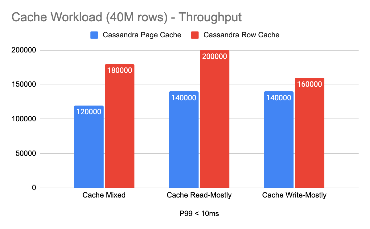
8779 Likewise, Figure 2 shows how throughput varies significantly
under a fully cached workload:
Figure 2 – Cassandra Row Cache vs OS Page Cache
performance (speedup falls between 1.14x to 1.5x)
Figure 2 – Cassandra Row Cache vs OS Page Cache performance
(speedup falls between 1.14x to 1.5x) An old
DataStax (IBM) documentation page strongly discourages its use,
noting that users should prefer using the OS page cache instead:
Note: Utilizing the appropriate OS
page cache will result in better performance than using row
caching. Counterintuitively, DataStax (IBM) later recommends
enabling the Row Cache when the number of reads dominate compared
to writes: Tip: Enable a row cache
only when the number of reads is much bigger (rule of thumb is 95%)
than the number of writes. Consider using the operating system page
cache instead of the row cache, because writes to a partition
invalidate the whole partition in the cache. OS Tuning
Operating system tuning for Cassandra shares many similarities with
other databases. Preventing swapping, tuning the kernel via
sysctl, setting disk read_ahead_kb
settings, configuring user limits and enabling Transparent
HugePages are the primary settings we touch when deploying
Cassandra. This is (undoubtedly) a non-exhaustive list, although it
should cover the strategies seen across most production Cassandra
deployments in practice. Depending on your setup, you may want to
further check: your
clocksource – particularly under Xen hypervisors; whether
cpupower supports setting the CPU scaling governor to
“performance” mode; experimenting with jemalloc;
configuring SMP IRQ
Affinity; and pinning Cassandra to specific CPUs via taskset(1).
Disks We primarily store Cassandra related files (including its
related logs) on locally-attached NVMe disks, as commonly found
within cloud hyperscalers. If there’s more than one attached disk
to the VM, we combine them into a RAID-0 array using
mdadm. In addition, we use XFS as the
backing filesystem, particularly as it’s the same we use for
ScyllaDB. We also set only one-hit merges, limit
read_ahead_kb to just 4kB, and disable
the IO scheduler (if any): MD_NAME=nvme1n1 sudo sh -c "echo 1
> /sys/block/$MD_NAME/queue/nomerges" sudo sh -c "echo 4 >
/sys/block/$MD_NAME/queue/read_ahead_kb" sudo sh -c "echo none >
/sys/block/$MD_NAME/queue/scheduler" Some important remarks:
the scheduler command may “fail” in modern Cloud
instances (and that’s fine); when using mdadm, tune
each block device individually backing the RAID device;
read_ahead_kb is a workload dependent setting. We
often test small partition lookups, but workloads with larger
wide-rows may benefit from increasing that setting. Memory We don’t
configure swapping at all to keep matters simple. The rationale is
that Cassandra already benefits from the OS page cache, and we
leave over half of the server’s RAM just for it. During our tests,
we also observed that enabling Transparent Huge pages,
especially with ZGC, contributed positively to
Cassandra’s performance. Although the improvement wasn’t
remarkable, we observed positive results similar to what both
Amy and
Netflix reported. The provided links already go in-depth on how
to enable THP, as well as how to configure Cassandra
to benefit from it. Keep in mind, however, that we recommend you
set the -XX:+AlwaysPreTouch JVM option regardless of
whether THP is enabled or not. That’s because it’s
known to improve overall JVM runtime performance at the expense of
increased JVM startup times. Kernel and User limits Put simply, you
don’t want Cassandra to be limited on either networking, memory
allocation, or the number of files it can open. We set
sysctl.conf.d/99-cassandra.conf to the following
values: net.ipv4.tcp_keepalive_time=60
net.ipv4.tcp_keepalive_probes=3 net.ipv4.tcp_keepalive_intvl=10
net.core.rmem_default=16777216 net.core.wmem_default=16777216
net.core.optmem_max=40960 vm.max_map_count = 1048575
net.ipv4.tcp_rmem = 4096 87380 16777216 net.ipv4.tcp_wmem = 4096
65536 16777216 net.core.rmem_max = 16777216 net.core.wmem_max =
16777216 net.core.netdev_max_backlog = 2500 net.core.somaxconn =
65000 net.ipv4.tcp_ecn = 0 net.ipv4.tcp_window_scaling = 1
net.ipv4.ip_local_port_range = 10000 65535 net.ipv4.tcp_syncookies
= 0 net.ipv4.tcp_timestamps = 0 net.ipv4.tcp_sack = 0
net.ipv4.tcp_fack = 1 net.ipv4.tcp_dsack = 1
net.ipv4.tcp_orphan_retries = 1 vm.dirty_background_bytes =
10485760 vm.dirty_bytes = 1073741824 vm.zone_reclaim_mode = 0
fs.file-max = 1073741824 vm.max_map_count = 1073741824
Lastly, the user running Cassandra must be allowed to allocate
enough resources for the process to run. As our VMs are
short-lived, we enable unlimited limits.conf
consumption to all users: * - nofile 1000000 * - memlock
unlimited * - fsize unlimited * - data unlimited * - rss unlimited
* - stack unlimited * - cpu unlimited * - nproc unlimited * - as
unlimited * - locks unlimited * - sigpending unlimited * - msgqueue
unlimited Parting Thoughts As demonstrated, Apache Cassandra
performance tuning is far from a one-size-fits-all solution. The
settings described throughout this article represent what worked
for our specific hardware setups and workload profiles. If your
deployment spans different hardware, many of the values presented
here will likely need to be revisited. This brings us to (perhaps)
the most underappreciated cost in Cassandra operations: dependency.
That is, every tuning decision is implicitly a contract with the
underlying hardware. Adding more disks, increasing CPU/RAM,
changing workloads are some overlooked aspects that will require
entirely new tuning cycles and re-evaluating your previous
decisions. ScyllaDB was designed with this problem in mind. Its
shard-per-core architecture and self-tuning capabilities
automatically adapt to the underlying hardware, eliminating much of
the manual iteration and tuning described here. There’s no JVM at
all, and most of the OS heavy lifting is carried out for you via an
automated script shipped alongside the core database. If Cassandra
performance has been a bottleneck, you’re concerned about the
recent IBM acquisition, or you’ve simply spent too much time
fighting tuning instead of building – give ScyllaDB a try. And if
you want to have a technical
discussion about your use case, let us know. “Key-Value” is Misleading. Access Patterns are Key.
Access patterns determine your data model, your I/O costs, and which database is the best fit for your workload I’ve been part of enough key-value database evaluations to recognize the pattern. When the conversation starts with benchmarks, the evaluation inevitably ends with regret. The benchmark answers “which is faster?” It doesn’t tell you which model fits how your application actually reads and writes data – and that’s what matters. Every data modeling decision should begin with access patterns, regardless of the technology on the table. What does your application read? At what granularity? What does it write? How often? How large? Let those answers drive the data model, then pick the technology. Flip that order and you pay for it. A fast database like ScyllaDB amplifies schema decisions: good models perform well, bad ones break faster. Edgar Codd invented First Normal Form (1NF) in 1970 to save disk space, but a terabyte of NVMe now costs about the same as lunch. So, even though the rule outlasted the constraint that justified it, we are still teaching it. That’s partly why so many teams expect to normalize their data with ScyllaDB the way they would a relational schema. But if they don’t get the order right (access patterns> data model> technology), they won’t get the performance that the engine was built to deliver. A lot of the confusion comes down to terminology. “Key-value” is one of the most overloaded labels in the database industry. We use it to describe both: A system that maps a string to an opaque blob A system that maps a partition key plus a clustering key to typed, individually addressable columns with partial-update semantics. Lumping these together hides the architectural decisions that determine your I/O patterns and your infrastructure costs. “Key-value” is often used to describe three very different data models. They differ in capability and in how deeply you can address your data. Pick the wrong one for your access patterns and you pay for it in I/O overhead, infrastructure cost, and write throughput. ScyllaDB can operate across multiple levels of this hierarchy. The one you select influences your I/O patterns, your update costs, and your infrastructure spend. Key-Value vs Wide-Column: Four Levels of Access Pattern Depth Instead of looking at feature lists, it’s better to compare these models by access pattern depth: at what level can you address, read, and write your data? Level 1: Key level. One key maps to one value. The value is opaque. The database has no knowledge of what is inside it. You get it and you put it in. This is K-V, the model behind most caching layers and session stores. Redis is the canonical example. The ceiling is the value boundary – you can replace it, you cannot address inside it. Level 2: Row level. A primary key maps to a set of named bins. Each bin holds a schemaless value. You can address individual bins by name, you can project specific bins in a read, and you can also update bins independently. This is K-V Wide Table, one key, multiple named fields, no schema enforcement on values. This model adds meaningful structure over K-V without requiring upfront schema design. Aerospike is the canonical example here. The ceiling is the bin boundary – you can update a bin, but you cannot address inside one. Level 3: Column level. A partition key combined with a clustering key addresses a row. Each column in that row is individually typed. The database understands the type of every value it stores. This is KKV Wide Table, the two-key model is what puts the second K in KKV. Typed columns enable the database to make smarter decisions about storage layout, compression, and update semantics. Cassandra reaches this level. The ceiling is the column boundary – typed and addressable, but complex values inside a column must be declared frozen. In other words, the entire value is serialized as a single blob that the engine cannot see into. Level 4: Within-column level. This is a key differentiator for KKV Wide Table. The engine starts working at a granularity that the other models can’t reach. A KKV Wide Table column can hold a collection: a map, a set, a list, a user-defined type, or nested combinations of these. Whether the database can address what’s inside that collection determines your actual access pattern depth. A frozen collection is serialized as a single blob. The engine stores it, retrieves it, and replaces it, but cannot see inside it. An unfrozen collection is stored element by element. Each entry is individually addressable. That distinction is the central architectural argument at this level. Cassandra touches this level but can’t reliably live here. Unfrozen collections exist in Cassandra, but tombstone accumulation makes them a liability in production. In ScyllaDB, Level 4 becomes practical. With an unfrozen collection, ScyllaDB stores each element individually. Whether you add an entry to a map, append to a list, or remove an element from a set – no read is required first and the database operates at element level. With a frozen collection, ScyllaDB serializes the entire value as a single cell. The engine can’t address inside it. For whole-value access patterns, that’s not a limitation, it’s an optimization. With this: There’s no per-element metadata. Reads pull one contiguous cell. Writes replace one contiguous cell. ScyllaDB’s UDT performance benchmarks show frozen collections outperforming unfrozen ones by up to 228% on write throughput and 162% on read throughput for 50-field UDTs. For the right access pattern, frozen is the faster choice. Don’t focus on frozen vs unfrozen; look at access pattern first and the right tool should follow from there. Figure: Frozen vs. unfrozen UDT, 50-field profile accessed as a whole. Frozen write throughput 228% higher, read throughput 162% higher. One cell write vs. 50-element writes plus 50 metadata records. The problem isn’t that it’s frozen; the access pattern mismatch is what’s causing the performance difference. An engineer who needs element-level updates and chooses frozen UDTs has, for those columns, given back Level 4 access. The operation degrades to read-modify-write: read the entire value, apply the change in memory, write it back as a whole. That is the same pattern a K-V Wide Table bin requires. The technology supports Level 4, but the schema choice has opted out of it. Figure: Four levels of access pattern depth. K-V gives key-level access. K-V Wide Table adds bin projection. KKV Wide Table adds typed columns and, with unfrozen collections, element-level access. Frozen collections are a performance optimization for whole-value access patterns, not a fallback. The opposite mistake is also a problem. An engineer who uses large unfrozen collections for values they always access as a whole pays per-element TTL and timestamp metadata on every element in the collection – at compaction time, continuously. A map with 10K entries carries 10K individual metadata records. That overhead snowballs over time. Choose frozen collections when you access the value as a whole. Choose small unfrozen collections when you need element-level updates. Large unfrozen collections are their own design smell, regardless of access pattern. Figure: Read granularity, requesting one field from a 30-field record. K-V reads the entire blob. K-V Wide Table reads the entire record and returns one bin. KKV Wide Table reads only the requested column, leaving 29 columns untouched on disk. How Access Pattern Depth Meets Memory: Three Scenarios The relationship between your dataset size and available memory determines which architecture is working with its strengths and which one is working against them. Figure: Data model behavior across memory scenarios, relative I/O and cost overhead for K-V, K-V Wide Table, and KKV Wide Table as dataset size moves from fits-in-RAM through keys-only-in-RAM to neither-fits-in-RAM. Scenario 1: Everything Fits in Memory When the entire dataset lives in RAM, a memory-resident hash index is fast. Point lookups are a hash computation and a pointer dereference. This is where K-V and K-V Wide Table architectures shine for read latency. But “what’s fast?” and “what’s cost-effective?” are different questions. If your dataset is 2 TB, you are paying for 2 TB of RAM across your cluster. An architecture designed around SSDs with efficient memory-resident metadata can deliver reads in the low hundreds of microseconds while your data lives on storage that costs a fraction of RAM per gigabyte. Although the access pattern performance difference on reads may be negligible, the infrastructure cost difference is not. Figure: Storage cost at scale, all-RAM vs NVMe SSD across dataset sizes from 0.5 TB to 32 TB. DDR5 ECC at ~$8/GB vs NVMe SSD at ~$0.10/GB. The gap compounds quickly past 1 TB. This is also the scenario where honesty matters. If your access pattern is truly “put blob, get blob” on ephemeral data with simple lookups, a K-V store is the right tool. The operational simplicity is a genuine advantage. There are fewer moving parts and fewer things to misconfigure. If your values are small and your queries never need to reach inside them, a K-V store will serve you well and be easy to operate. Scenario 2: Keys Fit in Memory, Values Do Not This is what K-V Wide Table architectures market as their sweet spot. Here, you have a primary index in memory, records on SSD, and fast key lookups that pull values from disk. For simple reads, bin projection works well here. Request three specific bins, get three bins back. You are not forced to read the entire record on every read. The problem surfaces at Level 4. Assume one bin holds a serialized map of user preferences and you need to update a single entry in that map. In this case, the system must: Read the entire bin from disk Deserialize the collection structure in memory Apply the modification Serialize the updated structure Write the entire bin back. That is a read-modify-write cycle on every collection update, regardless of how small the change is. The K-V Wide Table model has no path to Level 4 access. The bin is the floor. A KKV Wide Table model with unfrozen collections handles the same update without a read. The new map entry goes directly to the write-ahead log and the in-memory table. There’s no deserialization or full-bin read. The merge with existing data happens during compaction, as a background operation that does not block the write path. Compression: typed columns vs. schemaless bins. K-V Wide Table bins are schemaless. Within an SSTable block, different records interleave bin data without type information. That limits what a compressor can do across records. A KKV Wide Table stores typed column data within the same partition contiguously in SSTable blocks. For example, ScyllaDB writes all values for the event_ts column across rows in a partition together. Because those values share the same type, a dictionary-based compressor like zstd has much more to work with. This is not columnar storage in the analytics sense. ScyllaDB is an LSM-tree row-based engine at the partition level, not Parquet. The compression benefit comes from typed column homogeneity within SSTable blocks rather than a columnar storage layout. Frozen vs. unfrozen compression tradeoffs. Frozen UDTs compress well for a specific reason. A frozen UDT is a single cell with a consistent serialized layout. The same 50-field structure appears as the same byte sequence across records, which dictionary compression handles efficiently. Unfrozen collections are a different story. Each element carries its own TTL and timestamp metadata. ScyllaDB groups column values within SSTable blocks, which helps the element values themselves compress, but the metadata overhead scales with collection cardinality. For small unfrozen collections, it’s negligible. For large unfrozen collections, it can negate a meaningful portion of the compression gain. The compression advantage of typed columns applies most cleanly to simple typed columns and small unfrozen collections. Figure: K-V Wide Table SSTable blocks mix types across schemaless bins, limiting compression. KKV Wide Table SSTable blocks group typed column data within partitions. Frozen UDTs compress well as consistent serialized blobs. Unfrozen collections carry per-element metadata that can offset compression gains at high cardinality. Data locality. In a shard-per-core architecture (e.g., ScyllaDB’s), all columns within a partition live on the same CPU core. A read that touches three columns in a single partition involves zero cross-core coordination. This avoids locking and message passing between threads. This data locality might not be significant at low throughput. However, it matters a lot at hundreds of thousands of operations per second. Scenario 3: Neither Keys Nor Values Fit in Memory This is where memory-dependent index architectures hit a wall. If your architecture puts the primary index in RAM and your keyspace outgrows available memory, you are either: Adding nodes to hold the index, or Paging index entries to disk, which adds a disk read in front of every data read An architecture built for disk-resident data from the start does not have this problem. ScyllaDB (and to a degree Cassandra) uses Bloom filters to determine probabilistically whether a partition exists in a given SSTable without loading a full index into memory. Partition index summaries provide efficient lookup with a small, fixed memory footprint regardless of key count. And compaction strategies manage on-disk data organization to keep read amplification bounded. This is all strategic design for an architecture that assumes data will not fit in memory. Don’t just think about whether a system can handle disk-resident data; consider whether it was designed for it. The Update Path: Where Access Depth Becomes I/O Pattern Most evaluations obsess over reads. However, the update path is where access pattern depth differences tend to surface at scale. Consider updating a single element in a collection, one value in a map with 500 entries. In a K-V Wide Table architecture, collection updates require a full read-modify-write cycle: read the entire bin from disk, deserialize the collection structure in memory, apply the modification, serialize the updated structure, then write the entire bin back. Under concurrent updates to the same record, this becomes a serialization bottleneck. Under write-heavy workloads, write throughput is gated by read throughput. Figure: K-V Wide Table collection update path. A single-element update requires reading, deserializing, modifying, serializing, and rewriting the entire bin. In a KKV Wide Table architecture with unfrozen collections, the same update works like this: write the new value for that map entry directly to the memtable. This avoids the read, the deserialization, and the serialization. The entry lands in the write-ahead log and the in-memory table. The merge with existing data happens during compaction, as a background operation. Figure: KKV Wide Table update path with unfrozen collection. The write goes directly to WAL and memtable. No read required. Compaction merges data in the background. This is where access pattern honesty matters most. The append-only unfrozen update is fast for element-level changes to bounded collections. When your access pattern is whole-value, you write the entire UDT atomically and read it back as a unit. Here, frozen is the right choice. There is no read penalty and no per-element overhead. The ScyllaDB UDT benchmark shows 228% write throughput improvement for frozen UDTs in exactly this scenario: a 50-field UDT accessed and written as a whole. The frozen cell is one write operation. The equivalent unfrozen collection is 50 element writes plus 50 metadata records. The difference at 1,000 operations per second is negligible. But at 100,000 operations per second, with large collections and concurrent writes, the wrong frozen/unfrozen choice becomes the bottleneck in either direction. Figure: Write latency vs. collection size for a single-entry update. K-V Wide Table read-modify-write latency grows linearly with the number of entries in the collection. KKV Wide Table unfrozen update latency stays flat, the write goes to the WAL and memtable regardless of collection size. Figure: Single-element update latency vs. collection size, illustrating how wasted I/O grows with collection size for read-modify-write architectures, while direct-write latency remains constant. Choosing Honestly: Key-Value, K-V Wide Table, or KKV Wide Table These three models exist because different access patterns have different requirements. K-V is the right model for caching, session storage, and any workload where the access pattern is “put blob, get blob.” Its simplicity is a real advantage because you end up with fewer moving parts and fewer things to misconfigure. If your values are small and your queries never need to reach inside them, a K-V store will serve you well and be easy to operate. K-V Wide Table adds meaningful capability for workloads that need to address individual fields without upfront schema design. It’s a pragmatic choice for moderate-scale applications where operational simplicity matters, bin-level read projection is sufficient, and collection updates are infrequent or small. It sits at Level 2–3 access depth and does that job well. KKV Wide Table earns its complexity when your access patterns require Level 3 or 4 depth: frequent updates to large collections, datasets that will outgrow available memory, workloads where typed column compression meaningfully reduces storage cost, or write-heavy workloads that cannot afford read-modify-write on every collection update. The richer data model requires upfront schema design and demands that you get frozen versus unfrozen semantics right. Don’t rely on your intuition; choose strategically, based on your actual access pattern: Use frozen when you always read or write the whole value. A 50-field profile UDT that you always write and read back as a unit is a frozen candidate. The performance data supports it. Use small unfrozen collections when you need element-level updates. Append to a list. Update one key in a map. This is what unfrozen exists for. Use large unfrozen collections only if your access pattern is genuinely element-granular and your collection cardinality stays bounded. Per-element metadata overhead compounds. It affects both compaction cost and compression ratios. Figure: Decision flow for choosing a data model based on required access pattern depth. Don’t focus on which model is “best.” Think about which model best matches the access patterns your workload will experience in production. Start with the access patterns. Let the data model follow. Then pick the technology that supports that model at the depth you need. Get that order right and the database works with you. Get it wrong, and you spend your time working around it. *** If your use case requires low latencies at scale, and you’re frustrated with fighting your current database, ScyllaDB Cloud might be worth a look. Find me on LinkedIn – I’m always happy to talk data models.
What’s new in Cassandra® 6? A roundup of features for users and operators
Apache Cassandra 6 is shaping up to be significant release as some of its biggest changes affect the core behavior of the database:
- How metadata is coordinated
- How Cassandra is moving toward broader transaction support via Accord protocol
- How repair is scheduled, and
- How operators inspect and manage the system.
Let’s focus on a few changes that stand out:
- Accord transactions
- Transactional Cluster Metadata (TCM)
- Automated repair
- Constraints framework
- Zstandard dictionary compression, and
- Cursor-based compaction improvements.
Taken together, these changes point to a version of Cassandra that is becoming more structured internally and easier to operate.
Accord transactions for ACID guaranteesAccord is a general-purpose transaction framework that uses a leaderless consensus protocol to have highly available transactions and is used in Cassandra 6. The goal is broader transactional support across multiple keys, with strict serializable isolation and without a central bottleneck.
This matters because multi-key consistency is hard to handle cleanly in application code. Once a workflow spans more than one partition, the application often ends up doing coordination work that really belongs in the database.
Accord enables ACID behavior on transactional tables, which lets developers coordinate multi-step, multi-partition changes with stronger correctness guarantees, reducing the amount of custom consistency logic they have to build in the application.
Including multi-partition, conditional work has historically been difficult to express cleanly in Cassandra. For operators, it signals that transactions are becoming a more important part of the platform and something to watch closely as Cassandra continues to mature.
Read our deep dive on Accord transactions here.
Transactional Cluster Metadata (TCM)TCM changes how Cassandra coordinates cluster-wide metadata. TCM introduces a Cluster Metadata Service that keeps an ordered log of metadata changes and makes those changes visible in a more consistent, coordinated way. That includes things like membership, token ownership, and schema state.
This was introduced because Cassandra’s older model depended heavily on eventual consistency and the Gossip Protocol to spread metadata changes across the cluster. TCM is meant to make those changes more explicit, more ordered, and easier to reason about.
For operators, this is one of the biggest architectural shifts in Cassandra 6. It does not mean Gossip Protocol disappears everywhere, but it does mean Cassandra is moving away from Gossip as the primary way cluster membership, schema, and data placement changes are coordinated and made visible. For users, the result should be more predictable schema and topology operations.
Automated repair orchestrationAutomated repair brings repair orchestration into Cassandra itself. Repair is the mechanism Cassandra uses to reconcile replicas over time so they stay consistent, and the goal is to make repair scheduling and coordination a built-in database service rather than something operators must orchestrate with external tools.
This was introduced because repair is essential, but historically it has placed a real burden on operators. Teams have had to build their own schedules, decide how to run repair safely, and keep it consistent over time.
For operators, automated repair could be one of the most practical changes in the release. It reduces manual coordination, supports full and incremental repair, adds useful safeguards, and makes repair easier to treat as a normal part of cluster maintenance—just like it has happened with major compactions with Unified Compaction Strategy in Cassandra 5. For users, it means a better chance that maintenance happens regularly and with fewer gaps.
At NetApp Instaclustr, our expert TechOps team already orchestrates laborious tasks like repair for our Apache Cassandra customers, ensuring their clusters stay online. Our platform handles the complexity so you can get up and running fast.
Constraints framework for data validationThe constraints framework lets Cassandra enforce more targeted
validation rules as part of the table schema. It enforces them at
write time instead of relying entirely on application code to
reject invalid data. Some examples of constraints include: Scalar
(>, <, >=,
<=), LENGTH(),
OCTET_LENGTH(), NOT NULL,
JSON(), REGEXP().
A simple example of an in-line constraint:
CREATE TABLE users ( username text PRIMARY KEY, age int CHECK age >= 0 and age < 120 );
This was introduced because Cassandra already had some broad limits, but they were not very granular or expressive. The constraints framework gives teams a more precise way to protect the shape of their data and guard against bad writes from misconfigured clients.
Operators gain more control and better predictability around what gets written into the cluster. For developers, it means some validation can move closer to the schema instead of being duplicated across every service.
Zstd dictionary compressionZstandard, or Zstd, dictionary compression extends SSTable compression by letting Cassandra use trained Zstd dictionaries for repetitive data patterns. Instead of relying only on generic compression, it can use a dictionary built from representative data to improve results.
This was introduced to primarily improve compression ratio while keeping the design manageable in production. It is recommended to use minimal dictionaries and only adopt new ones when they’re noticeably better.
This makes compression more configurable and more visible for operators. It adds training workflows, dictionary lifecycle management, and observability into dictionary size and cached dictionary memory usage. For users, the main benefit is better storage efficiency, because data with strong repeating patterns can compress better, leading to potential performance gains.
You can read more about the constraints framework and Zstd dictionary compression in our article detailing recent CEPs.
Cursor-based compaction improvementsCursor-based compaction is a new low-allocation compaction path in Cassandra 6 that processes SSTable data in a more streaming-oriented way, using reusable cursor-like readers and writers instead of constantly creating large numbers of temporary in-memory objects. In practical terms, it is designed to reduce heap allocation and garbage collection overhead during compaction.
Compaction is one of Cassandra’s most important background processes, and when it becomes cheaper and more efficient, nodes can spend less time fighting garbage collection and less heap on temporary work. For operators, that can mean smoother performance and better efficiency on large datasets. For developers, it is mostly an under-the-hood improvement, but one that can help clusters behave more consistently under load.
Conclusion: A more manageable databaseWhat stands out about Cassandra 6 is that many of its biggest changes are not isolated features. They reshape core parts of how Cassandra behaves and how it is operated.
Accord introduces a broader transactional model. TCM changes how metadata is coordinated. Automated repair brings a core maintenance task into the database. Constraints make schemas more defensive. Zstd dictionary compression improves how Cassandra approaches storage efficiency, and cursor-based compaction makes the system easier to run.
Taken together, Cassandra 6 focused on making the database more deliberate internally and more manageable operationally.
Stay tuned for a preview release of Cassandra 6 on the Instaclustr Platform!
Ready to get started?If you want to experience the power of Apache Cassandra without the operational headache, we have you covered. If you are an existing customer and would like to try Cassandra 5 before 6.0 is released, you can spin up a cluster today. If you don’t have an account yet, sign up for a free trial and experience the latest generation of Apache Cassandra on the Instaclustr Managed Platform.
Read all our technical documentation here.
Discover the 10 rules you need to know when managing Apache Cassandra.
If you are using a relational database and are interested in vector search, check out this blog on support for pgvector, which is available as an add-on for Instaclustr for PostgreSQL services.
The post What’s new in Cassandra® 6? A roundup of features for users and operators appeared first on Instaclustr.
Introducing ScyllaDB Agent Skills
A new set of best practices and usage patterns for AI agents working with ScyllaDB Cloud clusters Today we’re releasing a curated set of best practices and usage patterns for AI agents working with ScyllaDB Cloud clusters. If you just want to grab the skills and go build, here you go:npx skills add
scylladb/agent-skills If you want to understand why these
skills are useful and what problems they solve, read on. ** You may
have noticed a short warning at the bottom of many AI applications:
“AI can make mistakes. Double-check the output.” Or something along
those lines. This is also true when it comes to working with
databases. We’ve seen agents reach for the wrong driver, fail to
connect to ScyllaDB Cloud, generate schemas that fit a relational
database but not NoSQL, and produce queries that technically
execute but perform poorly at scale.
For more on agents getting things wrong, see this video…These problems can all be minimized by using agent skills. What are Agent Skills? Agent Skills are markdown files that give your AI agent best practices and domain-specific knowledge. They follow the standard format and help your agent reduce hallucinations. They are also essential to give the agent up-to-date information. Since LLM training data doesn’t include real-time updates by default, these skills help bridge that gap. A specialized skill helps make the agent’s behavior more consistent and predictable. Available ScyllaDB Skills The ScyllaDB Agent Skills cover three distinct areas: scylladb-cloud-setup: Guides agents through the full connection flow: retrieving cluster credentials from the Cloud Console, selecting the correct shard-aware driver for the user’s language, configuring DC-aware load balancing with the right datacenter name, and verifying the connection. scylladb-data-modeling: Encodes query-first design methodology, partition key and clustering column patterns, anti-patterns (
ALLOW FILTERING, hot partitions,
unbounded partition growth), time-series bucketing, and guidance on
when to use secondary indexes versus denormalized tables. The goal
is to create schemas and queries that hold up under production load
(just returning correct results in development is not sufficient).
scylladb-vector-search: Covers vector index
creation, ANN queries, filtering strategies (global vs. local
indexes and when each applies), quantization, and driver
configuration. You can install all three at once, or pick only what
your project needs. Each skill loads on demand when a relevant task
comes up, they don’t interfere with each other. Let’s look at the
main areas where AI systems get ScyllaDB wrong. Shard-aware drivers
ScyllaDB has its own family of shard-aware drivers for Python,
Java, Go, Rust, C++, and
more. Agents sometimes decide to download the wrong driver.
While it may appear to work, unofficial drivers bypass ScyllaDB’s
shard-aware routing and degrade performance. In other cases, agents
may hallucinate non-existent drivers. Besides making it impossible
to connect to the ScyllaDB cluster, this also introduces a security
risk: you may install a fake package designed to trick the AI (this
is called slopsquatting).
Connecting to ScyllaDB Cloud Connecting to ScyllaDB Cloud requires
DC-aware load balancing configured with the exact datacenter name
(e.g. AWS_US_EAST_1) from your cluster. If your agent
gets that wrong, the driver will fail to connect. Data modeling
ScyllaDB’s data model requires you to have a query-first approach.
You design tables around your access patterns, not your entities.
Agents tend to be trained more heavily on SQL and relational
databases than on NoSQL systems such as ScyllaDB. That means they
are more likely to generate an entity-first schema, then use
ALLOW FILTERING to force queries. This can result in
suboptimal performance when using ScyllaDB. Vector Search Vector
search on ScyllaDB is powerful but specific. There are global and
local vector indexes with different filtering semantics and
performance considerations. There’s an ANN OF
operator, and quantization options that matter at scale. Choosing
the wrong index type for a filtered query can hurt performance.
Getting started Install all skills using the Vercel Skills CLI
(requires Node.js): npx skills add
scylladb/agent-skills Or install a specific skill: npx
skills add scylladb/agent-skills --skill
scylladb-data-modeling You can also install manually by
cloning the GitHub repository
and copying the skill folders into your agent’s skills directory:
Agent Skills directory Claude Code ~/.claude/skills/
Cursor ~/.cursor/skills/ OpenAI Codex
~/.codex/skills/ OpenCode
~/.config/opencode/skills/ The skills follow the
Agent Skills open standard
and work with any agent that supports it, including Claude Code,
Cursor, Codex, and GitHub Copilot. Native Claude Code and Cursor
plugins are coming soon. We recommend installing all three skills
in any project that uses ScyllaDB. You get full coverage of the
areas where agents most commonly go wrong, with no overhead when
those skills aren’t relevant to the current task. As of now, the
skills cover the CQL interface; Alternator (DynamoDB
API) is not yet included. Feedback is welcome. Create an
issue on GitHub!