The Evolution of Cassandra Data Movement at Netflix
By Guil Pires, Jennifer Prince, Jose Camacho, Ken Kurzweil, Phanindra Chunduru
Background
In a previous post, we introduced Data Bridge, a unified management plane for batch Data Movement at Netflix. Historically, several bespoke Data Movement connectors were developed across different engineering organizations to fulfill their specific requirements. Over the last few years, the Data Movement team has started centralizing these offerings through an abstraction that provides a catalog of connectors, along with simple UI and APIs to initiate Data Movement jobs.
One such case is the Cassandra to Iceberg connector. Apache Cassandra powers mission critical applications at Netflix, including Member, Billing, Recommendations, Subscriptions and many more. These use cases heavily leverage Data Movement to Apache Iceberg for many analytics and operational tasks, and central to this movement was a connector for Cassandra to Iceberg built in-house named Casspactor. As many Cassandra based Data Abstractions emerged, such as Key Value, Time Series and Graph — the need for larger and more complex Data Movement with transformations became more critical to the business.
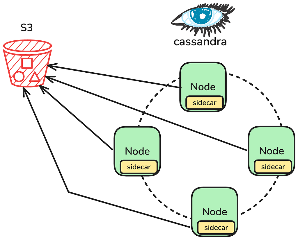
Data movements are fundamentally fulfilled by leveraging the existing Cassandra backup infrastructure. Regularly scheduled backups are performed directly on the Apache Cassandra nodes, via a sidecar process managing the upload of all necessary SSTables and associated Metadata files directly into Amazon S3. When a Data Movement job is initiated, the job constructs the specific backup structure it needs by referencing the S3 based metadata, allowing it to precisely locate the SSTable files. The engine then downloads these files, performs the required mutation compaction and processing, and finally writes the fully transformed, compacted data directly into the target Apache Iceberg tables.
Casspactor: The Engine We Outgrew
Casspactor processed roughly 1,200 data movements per day, transferring approximately 3 PB of data from Apache Cassandra into Apache Iceberg tables. It served some of the most critical workloads at Netflix. For years, it worked. Then, two compounding challenges made it clear we needed a fundamentally different architecture.
Fragile Metadata Dependencies
Before Casspactor could move a single record, it needed to answer a deceptively simple question: which backup exists, is it complete, and what does it contain?
Casspactor assembled this answer from multiple independent systems:
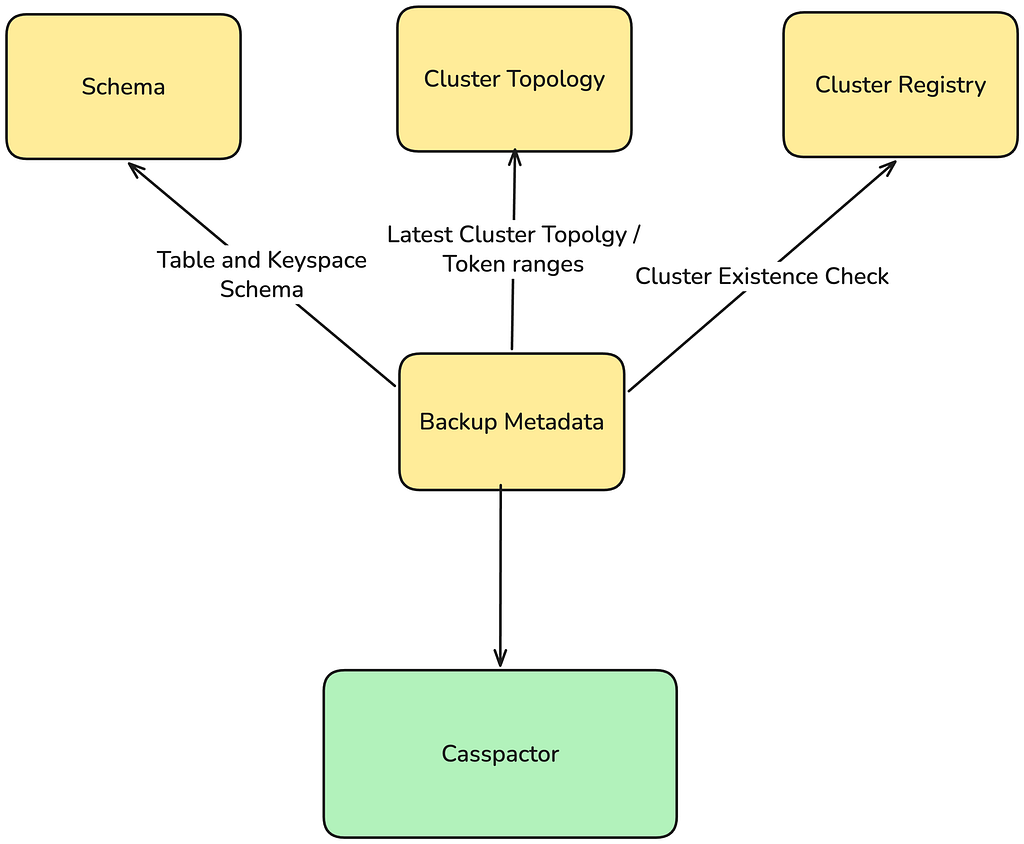
Each system had its own failure modes, update cadences, and accuracy guarantees. Casspactor’s view of the world was a composite, and composites diverge from reality.
Metadata fell out of sync with actual backups, causing Casspactor to read stale or incorrect data silently. Routine maintenance on the Cassandra Clusters triggered uncoordinated snapshots, and because Casspactor required all nodes in a region to snapshot at the same clock second, a single node replacement could break data movement for an entire region.
The fix was hiding in plain sight. The answer to “which backup exists and is it complete?” already lived in the backup storage layer (Amazon S3) itself. By reading metadata directly from the backup files, we could replace the entire dependency chain with a single source of truth.
Every Connector Inherited Casspactor’s Limitations
Cassandra at Netflix does not just store raw tables. It backs higher level data abstractions, such as Key Value, Time Series, and others, each with its own data model, access patterns, and semantics. When any of these abstractions needed to move data to Iceberg, they all funneled through Casspactor.
Every abstraction inherited Casspactor’s constraints:
- Skewed partition failures: Casspactor could not handle tables with large partitions, a common pattern in Key Value and Time Series workloads. Jobs crashed with out-of-memory errors on some of Netflix’s largest datasets.
- No data model awareness: Casspactor moved raw Cassandra tables as is. Connectors for Key Value and other abstractions had to bolt on post processing to reconstruct their data models from the raw output — extra cost, extra complexity, and an extra surface for failures.
- Intermediate table bloat: Casspactor wrote to an intermediate Iceberg table before producing the final output. The Key Value connector added another intermediate table and a snapshots table. Connectors for abstractions on top of Key Value added even more. This compounded into significant storage cost overhead.
- Inability to Time Travel: by relying on multiple services to compose a backup unit, Casspactor was unable to restore prior backups in the event of cluster Topology or Keyspace schema changes.
- Monolithic design: Casspactor was built as a single connector, not as an engine. There was no way to build a family of purpose built connectors on a shared foundation.
We needed something fundamentally different: an engine that reads directly from backups in S3, produces standard Spark DataFrames, and lets each data abstraction build its own connector with full awareness of its data model. One foundation, many connectors.
The New Stack: A Layered Architecture
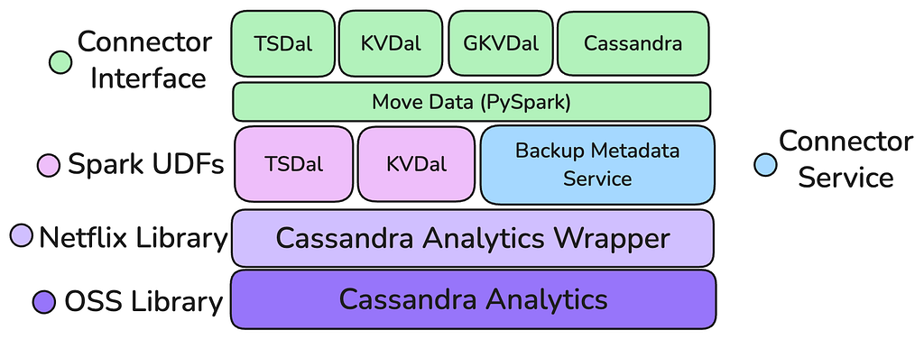
The new architecture, built upon the foundation of Apache Cassandra Analytics and the in-house Move Data framework, represents a fundamental shift toward a layered, purpose-built stack designed for reuse and maintainability. This new engine was conceived with clear separation of concerns, moving away from Casspactor’s monolithic design. The architecture is intentionally layered with the foundation being a core S3 reading capability: the Cassandra Analytics Wrapper, which is built on top of the Open Source Cassandra Analytics with Netflix’s internal backup representation and an S3 Client.
This layer handles the raw data retrieval from backups, translating it into standard Spark DataFrames. Sitting atop this foundation is a “Connector Factory” model, via both Java UDFs and transforms which allows individual data abstractions (Key Value, Time Series, others) to build highly optimized, data model aware connectors that process the generic Spark DataFrames, avoiding the need for complex, expensive, and failure-prone post-processing steps. This layered approach ensures that improvements to the core reading engine benefit all connectors, while the connectors themselves are focused solely on data transformation.
- Handles Skewed Partitions: By moving the mutation compaction and processing to the Executor level within Spark, the new engine can efficiently handle tables with highly skewed or wide partitions, a major pain point for Casspactor. Crucially, this processing occurs without excessive data shuffling, preventing out-of-memory errors and enabling reliable movement of Netflix’s largest datasets.
- Operates at Spark DataFrames (No Intermediary Tables): The new architecture directly generates standard Spark DataFrames from the Cassandra backups. This eliminates the need for Casspactor’s costly, multi-stage intermediate Iceberg tables, which led to storage bloat and operational complexity. This native DataFrame operation enables the “Connector Factory” by providing a universal, easily consumable interface for building diverse, model specific connectors.
- Jobs Auto Size: The engine integrates intelligent auto-sizing capabilities, allowing jobs to dynamically adjust resource consumption based on the source table’s characteristics. This removes the burden of manual tuning from engineering teams, ensuring optimal performance and cost efficiency without sacrificing reliability.
- Reduced Dependencies: By reading metadata directly from the backup files stored in S3, the new stack removes the fragile, multi-service dependency chain that plagued Casspactor. S3 becomes the single, authoritative source of truth for backup existence and completeness, vastly improving data movement reliability and consistency.
- Time Travel: A critical feature of the new stack is the ability to process the schema, cluster topology, and data as a cohesive unit at a specific point in time. This capability provides robust time travel functionality, essential for auditing, debugging, disaster recovery and reproducing past data states.
- Performance: Collectively, these architectural improvements, including native DataFrame processing, optimized partition handling, and streamlined metadata retrieval have resulted in notable performance gains, reducing overall data movement execution runtime and cost compared to the legacy Casspactor system.
- Cost: by eliminating intermediary Iceberg tables and efficient SSTable compaction on Executors, the new stack needs a significantly smaller storage and compute footprint leading to significant cost savings in the order of USD millions.
The Journey Towards a Safe Migration
The successful validation of the new stack was the critical first step, but it only marked the beginning of the most challenging phase: the migration. Large scale data migrations are inherently complex, high-risk undertakings that can be time consuming and often result in customer frustration and service disruption. To navigate the high stakes of decommissioning a mission-critical system like Casspactor and seamlessly replacing it, we needed a strategy that prioritized reliability and transparency above all else.
The migration was fundamentally enabled by a Like-for-Like strategy, which served as the cornerstone of our Platform Engineering philosophy, abstracting complexity. The core tenet was to maintain absolute consistency across the user-facing interface, the output contract, and the final data artifact. This meant ensuring that the data movement parameters defined via the Data Bridge abstraction remained unchanged, and, critically, the schema, metadata, and data within the destination Iceberg tables were identical to the legacy output. By preserving these external contracts, we eliminated the need for complex, time-consuming coordination with dozens of internal teams who relied on these data pipelines. This approach transformed the migration from a distributed, high-risk, multi-team effort into an internal platform implementation detail, allowing us to achieve a transparent, zero-impact transition and accelerate the retirement of the legacy system without requiring any code changes or validation from downstream users.
To navigate this migration, we developed a strategy anchored by three core pillars that serve as a blueprint for successful, large-scale data migrations:
- Validation: Establishing and maintaining absolute confidence in data consistency through rigorous, ongoing validation.
- Visibility: Instrumenting every part of the system to provide a clear, real-time understanding of migration progress and system health.
- Safety: Ensuring user impact is minimized or eliminated, despite the inevitable system failures, by leveraging abstractions and robust fallbacks.
The next section will provide a detailed exploration of these key pillars.
Pillar 1: Validation
Trust is earned, and in data migration, it is earned one row at a time. The first pillar is the most critical: providing a measurable guarantee to users and partners that the data produced by the new system is an exact, row-by-row replica of the data produced by the old one.
Our foundational tactic was deploying the new Move Data connector in a “shadow” testing that ran in parallel with the production Casspactor jobs. This allowed us to validate the new system with real-world, production workloads without any customer impact.
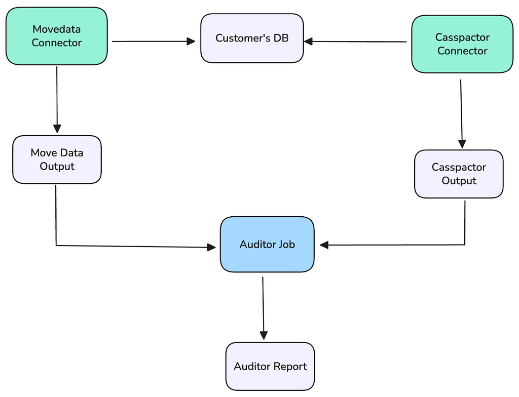
- Let C be the set of rows in the legacy Casspactor output (Iceberg table).
- Let M be the set of rows in the new Move Data output (Iceberg table).
The test for trust: prove that C = M. This required continuously checking for two conditions:
- Rows in C but not in M (C-M): The new system missed data.
- Rows in M but not in C (M-C): The new system introduced phantom or erroneous data.
Any result where the cardinality of these difference sets (the number of differing rows) was greater than zero triggered an immediate, high-priority investigation. The target was 100% similarity.
Uncovering and Resolving Disparities
The shadow mode quickly became a powerful forensic tool, exposing “unknown unknowns”, subtle discrepancies that were not bugs in the new system but rather differences in behavior between the new and old systems. Resolving these was the core work of building trust. For each problem we initiated an investigation log where we captured the details, logs, queries that allowed us to diagnose. Based on the assessment the issues were categorized so that similar differences on other datasets were later resolved affecting many of the shadow pipelines.
Maintaining an investigation log was critical to organize the outstanding issues and effectively communicate to stakeholders the progress and confidence of the new connector so that we effectively measure the appropriate level of “confidence” to initiate the migration.
We observed differences in how connectors leverage reference timestamps for Time-to-Live, Consistency Levels, backup selection, and various internal business logic. This continuous, data-driven cycle of discovery and resolution was the mechanism by which we built confidence in the new architecture.
Pillar 2: Visibility
Trust is built in the background, but an active migration requires real-time insight: Visibility. The second pillar involves instrumenting the system to provide an unambiguous, clear understanding of operational health and migration progress.
We extended our instrumentation to the overall migration workflow and its dependencies:
- Dashboards: We created centralized dashboards to track migration status, visualizing the total number of data movements migrated versus those remaining. The dashboards tracked execution status, average runtime, and cost comparisons between the two connectors.
- Dependency Tracking: Since the new system relied on a new set of APIs to fetch backup metadata, we implemented detailed metrics for failures to keep track of the APIs or dependencies failed.
- Alerting: Proactive alerts were set up for job failures (Move Data or Casspactor), failures on Move Data that triggered a fallback to Casspactor or any data discrepancy being detected.
This comprehensive instrumentation allowed the team to be proactive, fix issues as they emerged during the migration, and gain the necessary confidence to accelerate the migration timeline.
Pillar 3: Safety
Even with perfect data correctness and enhanced visibility, the third pillar, Safety is required for a zero-impact migration. The challenge is ensuring that when a system inevitably fails, the user experience is uninterrupted. Our strategy centered on decoupling the user’s workflow from the underlying connector implementation.
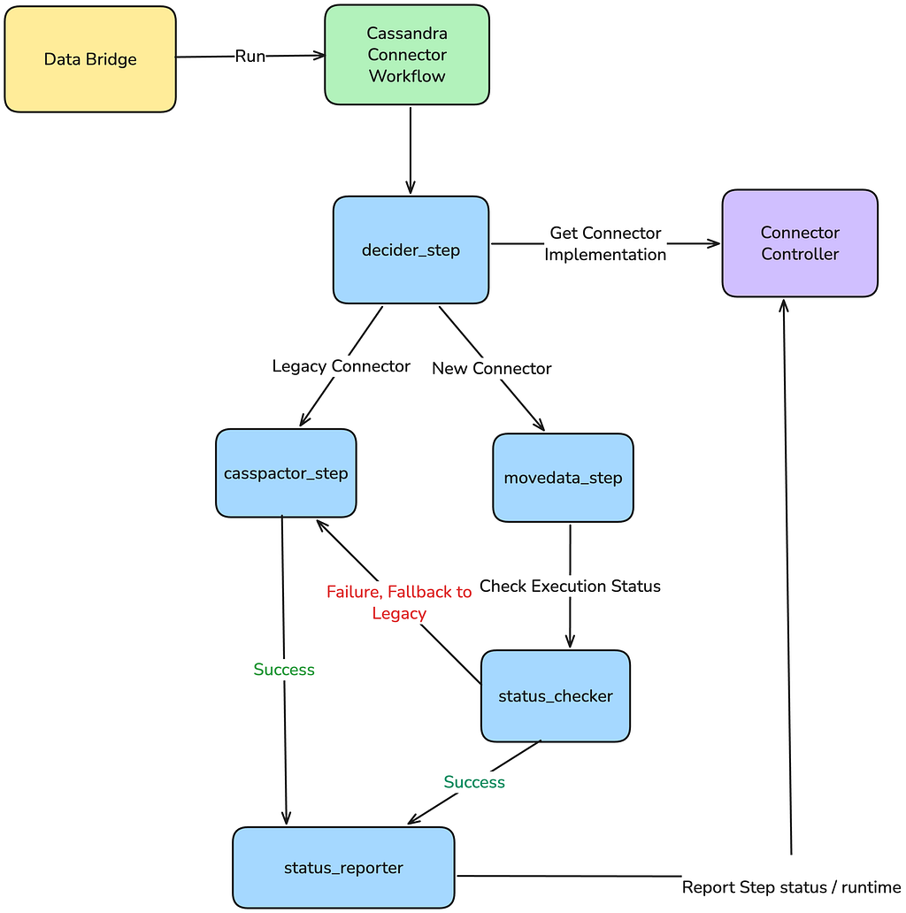
Leveraging Abstraction: The Decider Pattern
To achieve a transparent swap, we leveraged the Maestro workflow orchestration platform to implement the Decider pattern:
- Data Movement Abstraction: From a user’s perspective, their Data Movement job definition remained the same.
- The Decider Step: Internally the workflow responsible to execute the job was modified to include a Decider step. This step took the data movement parameters (source cluster, table name, destination) and invoked a control plane: Connector Controller.
- Connector Controller as the Registry: The control plane served as the dynamic registry. Based on the migration cohort and the data movement attributes, it determined and reported the appropriate connector to use either Casspactor (legacy) or Move Data (new).
This abstraction gave our team complete control. We could upgrade or rollback any connector for any data movement instantly by simply updating a configuration in the controller, with zero modification required to the thousands of downstream customer workflows. Crucially, this abstraction guaranteed the critical safety net: a conditional step in the Maestro workflow logic ensured that if the Move Data step fails, it would immediately execute the Casspactor step.
This pattern would increase the chances that the user’s data movement completes successfully, even if the new connector encountered a bug or transient failure during the initial rollout phases. User impact was completely eliminated; they might see a slightly longer runtime in the event of a failure and fallback, but they would never see a migration failure or suffer from stale data.
Beyond the workflow, the new system architecture itself was inherently more resilient. By building the new data movement connector on Cassandra Analytics and reading backups directly from S3, we removed fragile dependencies on deprecated internal services.
Conclusion
The migration from Casspactor to the new, layered architecture built on Cassandra Analytics and the Move Data connector was more than a typical “tech debt” project; it was a fundamental shift in our approach to data movement reliability and scalability at Netflix.
The legacy system, while serving us well for years, was ultimately constrained by monolithic design, fragile metadata dependencies, and an inability to handle the complexity of modern data abstractions. The new stack resolves these issues by delivering a robust, cost-efficient, and inherently more resilient solution that reads directly from S3, handles wide partitions gracefully, and eliminates costly intermediate tables.
Our blueprint for the migration, anchored by the three pillars of Validation, Visibility, and Safety, ensured a transparent and high-confidence transition. Through rigorous shadow testing and a data-driven audit framework, we achieved the desired data consistency. Enhanced dashboards and alerting provided the real-time operational insight necessary to manage risk. Most critically, the implementation of the Decider pattern within our workflow abstraction minimized the impact for all downstream users.
This successful migration validates a core philosophy: by abstracting complexity at the platform level, we can perform large system migrations without burdening our product engineering partners. The new foundation is now ready to support the next generation of Netflix’s data abstractions.
Looking ahead
This foundational work on the Cassandra Data Movement stack has done more than just replace a legacy system: it has become an accelerator for innovation across the entire Data Movement organization. By providing a reliable, performant engine that standardizes data retrieval into Spark DataFrames, we’ve enabled the rapid development of new, highly optimized connectors. This new “Connector Factory” approach has already delivered a dedicated Key-Value to Iceberg and Time Series connectors, both of which are fully aware of their respective data models, eliminating costly post-processing. This architecture is also paving the way for ambitious new initiatives, including the development of a solution for bulk loading data into Cassandra itself, effectively completing the data movement cycle, and enabling safer fleetwide connector rollout with canaries inspired by the Decider Pattern.
We are incredibly grateful for the extensive collaboration among the Data Movement, Data Bridge, Online Data Stores, Membership, Billing, Subscriber and Ads platform teams at Netflix; this work simply couldn’t have been accomplished without their partnership!
The Evolution of Cassandra Data Movement at Netflix was originally published in Netflix TechBlog on Medium, where people are continuing the conversation by highlighting and responding to this story.
Instaclustr product update: June 2026
Here’s a roundup of the latest features and updates that we’ve recently released.
If you have any particular feature requests or enhancement ideas that you would like to see, please get in touch with us.
Major announcements AI Search for OpenSearch is now generally available on the NetApp Instaclustr Managed PlatformAI Search for OpenSearch is generally available on the NetApp Instaclustr Managed Platform. It brings semantic search, hybrid search, and retrieval-augmented generation (RAG) without the complexity of managing software, infrastructure, or operational management. General availability expands on the public preview, adding support for external LLM and embedding services such as Amazon Bedrock and OpenAI for enterprise search, e-commerce, support chatbots, and observability-style use cases. Unlock new possibilities with AI search—learn more.
Introducing Kafka Client Telemetry: Centralized client metrics for Instaclustr Managed Apache Kafka®NetApp is introducing Client Telemetry for Instaclustr for Apache Kafka®, designed to deliver broker-integrated visibility into Kafka client and application-level metrics, with telemetry export and centralized collection. Instaclustr for Apache Kafka users can gain visibility into client behavior such as connection status, request rates, error rates, and latency from the broker, simplifying monitoring and supporting a holistic view of client interactions. Compliant Kafka clients collect metrics and push them to the brokers; brokers use an OpenTelemetry Collector to forward metrics to a customer-specified destination, with Prometheus 3.0+ and Datadog supported in this initial release.
Powering low-latency analytics with ClickHouse® and Amazon FSxInstaclustr Managed ClickHouse integrated with Amazon FSx for NetApp ONTAP is built to run analytical queries directly on file-based data that can transparently tier to lower-cost capacity, without relying on extra staging layers, ingestion pipelines, or format-specific copies to make data queryable. The integration now supports deployments where compute and storage can reside in different VPCs or AWS accounts, enabling flexible, enterprise-grade architectures with consistent storage access across network and account boundaries.
Other significant changes Apache Cassandra®- Self-service iccassandra password reset — customers can now reset their iccassandra database password directly from the console via the Connection Info page, eliminating the need to raise a support ticket. The new password is displayed for 5 days before being automatically removed.
- Released Apache Cassandra v4.1.10 into General Availability on the NetApp Instaclustr Managed Platform, delivering a stability-focused patch release, while deprecating Apache Cassandra 4.1.9.
- Kafka and Kafka Connect 3.9.2 released to General Availability.
- Kafka and Kafka Connect 4.1.2 released to General Availability.
- Karapace Schema Registry 5.2.0 and Karapace Rest Proxy 5.2.0 are added support for Kafka clusters.
- ClickHouse v25.8.24 released to General Availability.
- New c7g.8xlarge node size on the AWS provider has been added to support OpenSearch clusters.
- OpenSearch 3.5.0 released to General Availability.
- AI Search is now available on the free trial.
- PostgreSQL 18.3, 17.9, and 16.13 and PgBouncer 1.25.1 released to General Availability.
- The new AWS region, ap-southeast-6 (New Zealand), has been added.
- Cluster tag management improvements — multiple enhancements to tag search, display, and validation in the console and API, including prevention of duplicate tag keys for better data consistency.
- We’re preparing to introduce GPU nodes for OpenSearch on the NetApp Instaclustr Managed Platform, bringing dedicated machine learning capabilities directly into your managed clusters. With GPU nodes, vector indexing can be up to 10x faster and CPU load is reduced, freeing cluster capacity for mission-critical workloads. Additionally, GPUs offer superior cost-efficiency compared to traditional CPU-based vector indexing, driving down the total cost of ownership.
- We’re close to launching PostgreSQL® integrated with FSx for NetApp ONTAP (FSxN) into GA, now including NVMe support—designed to deliver improved throughput, up to 20% observed greater throughput than we achieved with our public preview. This enhancement combines enterprise-grade PostgreSQL with FSxN’s scalable, cost-efficient storage for better cost, performance, and flexibility, while enabling ONTAP snapshots for backups, mirroring, and multi-region recovery—fast snapshot/restore and daily backups for large databases.
- NetApp Instaclustr plans to release the Remote MCP Gateway Service powered by AgentGateway on the Instaclustr Managed Platform. This service will let you, in minutes, provision and configure a production-ready Model Context Protocol gateway to provide LLM access to databases, application data infrastructure services, and REST APIs.
- Coming soon, NetApp Instaclustr will be launching the
Self-Service Bring Your Own Cloud (BYOC) feature for AWS, offering
a fully guided onboarding experience that allows customers to
connect their AWS accounts and begin deploying managed clusters
directly from the console — making it faster and easier for
customers who prefer to run clusters in their own cloud
environments.
Cluster DNS will soon be available for Apache Cassandra and Apache Kafka clusters on AWS allowing you to connect to your applications using simple, stable hostnames instead of long lists of IP addresses. When node IPs change due to scaling, replacement, or maintenance there is no longer a need to update client configuration.
- Need an end-to-end pattern for streaming analytics on AWS? The same-day three-part series How to build a streaming analytics pipeline with Terraform and Instaclustr, Part 1: Setting up your first Kafka® cluster, Part 2: Designing the complete data pipeline, and Part 3: Integrating with AWS VPC show how to stand up Kafka with Terraform, connect ClickHouse and Kafka Connect into a real pipeline, and finish with VPC integration for secure networking. Together the posts bridge provisioning, data flow design, and cloud networking without skipping the glue work that usually stalls proof-of-concepts.
- Apache Kafka 4.1.0 introduces the Streams Rebalance Protocol in early access for Kafka Streams: a broker-driven assignment model that eliminates client-side coordination, reduces “stop-the-world” rebalance pauses, and delivers smoother task assignment as Streams applications scale horizontally. For a walkthrough of when you need it, how to enable it, and what to expect, see What’s new in Kafka® 4.1.0? Introducing the new Streams Rebalance Protocol.
- OpenSearch 3.6 release bundles a wide set of upstream changes: ML Commons AI agent improvement such as token usage tracking, k-NN vector search performance improvements including Lucene Better Binary Quantization, Dashboards updates across AI chat and Explore, and OpenSearch APM for observability. For a single walkthrough of those themes, see OpenSearch version 3.6 release: smart agents and fast search. We’re currently testing OpenSearch 3.6 for compatibility and security purposes. Keep an eye on our release blog for more information about when this exciting new release will be available on the managed platform.
If you have any questions or need further assistance with these enhancements to the Instaclustr Managed Platform, please contact us.
SAFE HARBOR STATEMENT: Any unreleased services or features referenced in this blog are not currently available and may not be made generally available on time or at all, as may be determined in NetApp’s sole discretion. Any such referenced services or features do not represent promises to deliver, commitments, or obligations of NetApp and may not be incorporated into any contract. Customers should make their purchase decisions based upon services and features that are currently generally available.
The post Instaclustr product update: June 2026 appeared first on Instaclustr.
Automate ScyllaDB X Cloud Clusters with Terraform
The ScyllaDB Cloud Terraform provider gives you infrastructure-as-code control over your clusters The ScyllaDB Cloud Terraform provider now supports ScyllaDB X Cloud. That means you can provision and manage elastic, autoscaling ScyllaDB clusters the same way you manage the rest of your infrastructure. The ScyllaDB Cloud Terraform Provider The provider lives atregistry.terraform.io/scylladb/scylladbcloud. You need
a ScyllaDB Cloud account and an API token from cloud.scylladb.com.
terraform { required_providers { scylladbcloud = { source =
"registry.terraform.io/scylladb/scylladbcloud" version = "~>
0.3" } } required_version = ">= 0.13" } provider "scylladbcloud"
{ token = var.scylladb_token }
Pass the token through a
variable. What Is ScyllaDB X Cloud? ScyllaDB X Cloud is
ScyllaDB’s elastic cluster tier built on a tablets-based
architecture. Traditional ScyllaDB clusters use token ranges pinned
to nodes. Scaling them up or down means rebalancing large chunks of
data. X Cloud uses tablets, which are smaller, independently
moveable units of data. When you add or remove nodes, tablets
rebalance in parallel across the cluster, which makes scaling fast
and non-disruptive. In practice this means you can: Scale from 100K
to 2M ops/sec in minutes, not hours Push storage utilization up to
90% before scaling out (no wasted headroom) Scale-in when load
drops (pay for what you use) X Cloud also differs from standard
clusters in how you configure it in Terraform: instead of choosing
a fixed node type and count, you define a scaling
policy and let the platform decide the right size.
Provisioning an X Cloud Cluster Here is a complete cluster
resource: resource "scylladbcloud_cluster" "xcloud" { name =
"my-xcloud-cluster" cloud = "AWS" region = "us-east-1" cidr_block =
"172.31.0.0/16" scaling { instance_families = ["i8g"]
storage_policy { min_gb = 500 target_utilization = 0.75 }
vcpu_policy { min = 6 } } } The scaling block
is what makes this an X Cloud cluster. It is mutually exclusive
with the node_type and min_nodes fields
used by standard clusters (you use one or the other). Key Scaling
Parameters instance_families instance_families =
["i8g"] X Cloud scales within a single instance family. The
platform picks specific instance sizes within that family as load
changes. Sticking with instance_families rather than
listing explicit instance_types gives the autoscaler
more room to work with. If you do restrict it to specific types,
allow at least three different types to give the scaler meaningful
options. storage_policy.min_gb storage_policy { min_gb = 500
} The cluster will not scale below this physical storage
threshold. Set it when you know your dataset has a minimum size and
want to avoid scale-in churn. storage_policy.target_utilization
storage_policy { target_utilization = 0.75 } This is
the utilization level the autoscaler aims to maintain. The valid
range is 0.7–0.9 (default: 0.8). The scaler adds capacity when
utilization exceeds target by more than 5%, and removes capacity
when it falls more than 5% below target. For write-heavy workloads,
staying below 0.85 is a good baseline. It gives compaction and
repairs room to breathe. vcpu_policy.min vcpu_policy { min =
6 } The cluster will not scale below this vCPU count,
regardless of load. That’s good for latency-sensitive workloads
where you want compute headroom even at low traffic. Standard
Clusters (For Comparison) If you need a fixed-size cluster or
require multi-DC deployments (which will be supported soon), use
the standard configuration: resource "scylladbcloud_cluster"
"standard" { name = "my-standard-cluster" cloud = "AWS" region =
"us-east-1" node_type = "i3.large" min_nodes = 3 cidr_block =
"172.31.0.0/16" } Standard clusters use
node_type and min_nodes instead of a
scaling block. Outputs After apply, the provider
exposes: output "cluster_id" { value =
scylladbcloud_cluster.xcloud.cluster_id } output "datacenter" {
value = scylladbcloud_cluster.xcloud.datacenter } output
"node_dns_names" { value =
scylladbcloud_cluster.xcloud.node_dns_names }
node_dns_names provides the hostnames to pass to your
driver configuration. Wrapping Up The ScyllaDB Cloud Terraform
provider gives you infrastructure-as-code control over your
clusters. For X Cloud specifically, the scaling block
replaces the manual node sizing decisions. You just define the
baselines and the platform handles the rest. ScyllaDB’s
tablets-based architecture means scale events are fast enough to
respond “just-in-time” to real traffic changes – so you don’t need
to overprovision for peak capacity just in case. For more details,
see the full provider documentation at
registry.terraform.io/providers/scylladb/scylladbcloud. ScyllaDB Customer Experience Spotlight: Faisal Saeed
Welcome to the second installment of a new blog series introducing some of the experts you might encounter when you work with ScyllaDB. (In the first, we met Tyler Denton, Solutions Architect). Today we’re featuring Faisal Saeed, Principal Customer Engineer on the Customer Experience team here at ScyllaDB. He lives in Singapore and has been at ScyllaDB for more than 2 years. Let’s learn a little about Faisal… What do you do here at ScyllaDB I have a hybrid role where I work with existing customers as their Principal Customer Engineer, helping them ensure their ScyllaDB Cloud / on-prem clusters are in good health and performing according to their expectations. Secondly, I work as a pre-sales Solutions Architect for clients who are not existing ScyllaDB customers and are evaluating ScyllaDB. Here, I often help with data modeling or planning their data migration from their existing database into ScyllaDB Enterprise / ScyllaDB Cloud clusters. Please share a little about your path to ScyllaDB I have worked in the IT industry for about 30 years and have extensive database experience. Before joining ScyllaDB, I was a Principal Solutions Architect with MariaDB for 6 years. Before that, I worked with ACI Worldwide as a database architect on projects for DBS Bank in Singapore. Before that, I spent many years at NCS, working as a database architect on DBS Bank projects. Tell me about one of the most interesting projects you’ve worked on here While I work with many amazing customers, the project I cherish the most is an in-house developed tool that automates ScyllaDB Enterprise/Cloud/X Cloud clusters with a single command, allowing the user to run various workloads and perform stress testing of multiple clusters. This is the ScyllaDB Automation Framework, and I have worked on this project for more than a year. This helps various team members in ScyllaDB with their day to day tasks, whether running a demo for a customer or simulating a customer use case. What’s the most impressive ScyllaDB feat you’ve seen a team accomplish If we talk about teams in ScyllaDB, X Cloud is an amazing ScyllaDB product that lets customers save costs while running at any scale. The team has done an outstanding job. Talking about customers, every one of them is unique in some way. JioStar from India uses ScyllaDB to support IPL, World Cup Cricket, and many other supporting events where millions of users concurrently log in to ScyllaDB clusters through their app — and ScyllaDB handles them gracefully without any lags. There are many others, but I can’t mention everyone. What do you like to do when you’re not working or on-call I spend time with my wife at home, go out for long walks, watch movies, and care for two bunnies who have been with us for more than 5 years. What’s your top tip for getting the most out of ScyllaDB I can’t recommend just one thing, but ScyllaDB is designed to run almost on autopilot. Rarely is there a need to tune any aspect of the ScyllaDB cluster. But if I had to pick one thing, it would be “proper NoSQL data modeling.” I have seen many teams struggle with performance because they had a poor data model. After spending some time with them and helping them fix their data model mistakes, their ScyllaDB cluster ran smoothly with the promised single-digit P99 latencies. I recommend everyone to join ScyllaDB University (it’s free) and take the beginner and advanced data modeling courses.ScyllaDB Operator 1.21 Release — with Oracle Kubernetes Engine (OKE) Support
Introducing Oracle Kubernetes Engine support, stronger TLS, and a lighter dependency footprint ScyllaDB Operator 1.21.0 is now available. For background, ScyllaDB Operator is an open-source project that helps you run ScyllaDB on Kubernetes. It lets you manage ScyllaDB clusters deployed to Kubernetes and automate tasks related to operating a ScyllaDB cluster (e.g., installation, vertical and horizontal scaling, as well as rolling upgrades). ScyllaDB Operator 1.21 expands cloud platform support with OKE, adds ECDSA as an alternative key type for TLS certificates, and removes a hard dependency on Prometheus Operator. Oracle Kubernetes Engine (OKE) support ScyllaDB Operator 1.21 adds Oracle Container Engine for Kubernetes (OKE) as a supported platform. The new OKE support comes with comprehensive documentation covering the entire workflow , from provisioning the underlying OCI infrastructure (VCN, subnets, gateways, and node pools with Dense I/O shapes and local NVMe storage) to deploying a 3-node ScyllaDB cluster spread across fault domains. An automated setup script is also provided for one-command infrastructure provisioning. To get started with ScyllaDB on OKE, see the Set up an OKE cluster for ScyllaDB infrastructure guide and the OKE reference deployment. ECDSA support for TLS certificates ScyllaDB Operator manages TLS certificates internally for securing client-to-node communication. Until now, only RSA keys were supported for certificate generation. ScyllaDB Operator 1.21 adds elliptic curve cryptography (ECDSA) as an alternative key type. This allows smaller key sizes and faster cryptographic operations with strong security. You can opt in to ECDSA by setting the –crypto-key-type=ECDSA flag on the operator, with the curve bit-size configurable via –crypto-ecdsa-key-size (defaulting to P-384). RSA remains the default key type. The RSA key size is now configured with a dedicated –crypto-rsa-key-size flag; the previous –crypto-key-size flag is deprecated and remains accepted as an alias. Prometheus Operator is now an optional dependency Previously, ScyllaDB Operator required Prometheus Operator CRDs (monitoring.coreos.com/v1) to be installed in the cluster, even if you did not intend to use ScyllaDBMonitoring. Missing CRDs would result in error logs at startup. With ScyllaDB Operator 1.21, Prometheus Operator becomes a purely optional dependency. The operator auto-detects whether the CRDs are present at startup using Kubernetes API discovery. When they are absent, the ScyllaDBMonitoring controller is not started and no error logs are emitted. If you install Prometheus Operator after the ScyllaDB Operator is already running, restart the operator to pick up the new CRDs. Refer to the monitoring setup guide for details.
Using Salting to Lower Latency for Large Blobs in ScyllaDB
A modified salting technique that cuts P99 write latency 22x for large blobs Storing huge blobs in any database has always been, and still is, very challenging. Large allocations required for storing, reading, compacting, and repairing such cells always create significant pressure on the memory allocation sub-system. In addition, receiving a write request or sending a read response with a huge payload on a shared connection creates a “head of line” issue impacting the latency of other requests. This is true for every database! Consequently, by splitting the blob into smaller chunks and processing them in parallel, we can achieve latencies comparable to a single chunk read/write operation. Naturally, when all your data consists of huge blobs, you are probably not going to use CQL or SQL databases to store them. You will use S3-like storage for blobs and will use CQL/SQL DB to store references to those blobs. However, if your data is mostly reasonably small but has a small part of the population that are huge blobs, you may want to be able to serve both small and large blobs from the same database. While working with ScyllaDB, we found that a modified salting technique can address the latency impact of storing large blobs. In this post, we present that salting technique, then explain when/how to apply it. Background: Large Blobs in ScyllaDB For a better idea of how storing large blobs impacts performance, let’s look at an example. In our testing of ScyllaDB version 2026.1.1 with cassandra-stress tool, we observed that writing key-value rows with a 60MB blob cell results in an average latency of about 568ms and P99 latencies of 1.4s. In contrast, writing K/V data of 1MB yields an average latency of 2.2ms, with a P99 of approximately 4.5ms. When writing 60MB cells, ScyllaDB could not go any faster because its memory management system was totally saturated. Below are the results of the 60MB cell test (with a single i8g.4xlarge node): Results:Op rate : 18 op/s [WRITE: 18 op/s]
Partition rate : 18 pk/s [WRITE: 18 pk/s] Row rate : 18 row/s
[WRITE: 18 row/s] Latency mean : 567.6 ms [WRITE: 567.6 ms] Latency
median : 497.0 ms [WRITE: 497.0 ms] Latency 95th percentile :
1087.4 ms [WRITE: 1,087.4 ms] Latency 99th percentile : 1436.5 ms
[WRITE: 1,436.5 ms] Latency 99.9th percentile : 1874.9 ms [WRITE:
1,874.9 ms] Latency max : 1995.4 ms [WRITE: 1,995.4 ms] Total
partitions : 1,000 [WRITE: 1,000] Total errors : 0 [WRITE: 0] Total
GC count : 0 Total GC memory : 0.000 KiB Total GC time : 0.0
seconds Avg GC time : NaN ms StdDev GC time : 0.0 ms Total
operation time : 00:00:55 And here are the results of writes
of 1MB cells with the same rate byte-to-byte with the 60MB
execution above: Op rate : 1,061 op/s [WRITE: 1,080 op/s]
Partition rate : 1,061 pk/s [WRITE: 1,080 pk/s] Row rate : 1,061
row/s [WRITE: 1,080 row/s] Latency mean : 2.2 ms [WRITE: 2.2 ms]
Latency median : 2.0 ms [WRITE: 2.0 ms] Latency 95th percentile :
2.8 ms [WRITE: 2.8 ms] Latency 99th percentile : 4.5 ms [WRITE: 4.5
ms] Latency 99.9th percentile : 15.0 ms [WRITE: 15.0 ms] Latency
max : 41.6 ms [WRITE: 41.6 ms] Total partitions : 60,000 [WRITE:
60,000] Total errors : 0 [WRITE: 0] Total GC count : 0 Total GC
memory : 0.000 KiB Total GC time : 0.0 seconds Avg GC time : NaN ms
StdDev GC time : 0.0 ms Total operation time : 00:00:56 The
60MB blob results are suboptimal for high-performance requirements.
However, 1MB results show that if we can split the blob into
smaller chunks and write/read them in parallel we can achieve
latencies close to a single chunk read/write operation. Perhaps
salting can help us achieve this? Classic Salting Technique The
classic “salting” technique, used to break down large partitions
consisting of too many rows, introduces an additional “salt” column
to the partition key. It selects a random value from a known range
(e.g., an integer between 0 and 99) to store the next row. This
will distribute what once was a single large partition for a key
KEY1 into 100 smaller partitions with partition keys (KEY1, 0),
(KEY1, 1) …, (KEY1, 99) each of about 1/100 the size of the
original one. The primary drawback of this technique for large
partitions is the necessity of using “salting” for every row, as
the system does not inherently know if a row belongs to a large
partition. Consequently, reading data for any original key KEYn
requires reading all 100 partitions (KEYn, k), where k=0, 1, …, 99.
And this may be very wasteful because large partitions normally
represent a very small part of the total partition population.
Similarly, large blobs typically represent only a small fraction of
the total blob population. Another “weak spot” of the classic
“salting” is that you can’t reduce the SALT cardinality — you can
only increase it. This means that if the size of your large
partitions got smaller, you would still need to use the same “salt”
cardinality you already used before. Modified Salting Technique for
Storing Blobs We found that improving the original “salting”
algorithm for a blob case can eliminate both of those drawbacks.
Let’s look at how we modified that classic salting technique.
Schema Let’s assume that the original table schema is as follows:
CREATE TABLE keyspace1.standard1 ( key blob, value blob,
PRIMARY KEY (key) )
For our algorithm, we modify it to:
CREATE TABLE keyspace1.standard1 ( key blob, salt int,
chunk_id int, chunk blob, total_chunks int, salt_cardinality int
PRIMARY KEY ((key, salt), chunk_id) )
Algorithm Write On a
write path, we are going to store the used “max_salt”
(salt_cardinality) and the total number of chunks
(total_chunks) in every row in addition to the rest of the
chunk-specific data for simplicity. If you want to optimize the
storage to a bitter end, you can store salt_cardinality
and total_chunks only in the “metadata row” (see below).
def write_key_blob(key, blob, max_salt=100,
max_chunk_size=4096): # Split blob into chunks; last chunk may be
smaller split_blob_chunks: List[bytes] = split_blob(blob,
max_chunk_size) num_chunks = len(split_blob_chunks)
salted_partition_chunks = [[]] * min(num_chunks, max_salt) for
chunk_id, chunk in enumerate(split_blob_chunks):
salted_partition_chunks[chunk_id % max_salt].append( (chunk_id,
chunk) ) for salt, chunks in enumerate(salted_partition_chunks): #
Inserts salted partition in one or a few UNLOGGED BATCHes
insert_async_batch( key=key, salt=salt, chunks=chunks,
total_chunks=num_chunks, salt_cardinality=max_salt )
Complexity Memory: O(sizeof(blob)) CPU:
O(num_chunks) DB:
O(num_salted_partitions), where
num_salted_partitions = min(num_chunks, max_salt) Latency Maximum
batches concurrency divided by the num_salted_partitions times the
single batch latency. If all batches can be sent out in parallel,
the whole write is going to take the time it takes to write a
single salted partition data. Read On a read path, we are going to
start with reading total_chunks and
salt_cardinality from the “metadata row” of a specific
Key: row with (key=Key, salt=0, chunk_id=0) primary key. If we have
stored any data for the Key, this row should exist. Once we have
total_chunks and salt_cardinality values, we can
calculate primary key values for every chunk of the original blob
we stored before, and read them all in parallel. Below you can find
a pseudo-code implementing this idea. def read_key_blob(key:
bytes): # SELECT (total_chunks, salt_cardinality) FROM
keyspace1.standard1 # WHERE key=key AND salt=0 AND chunk_id=0
total_chunks, max_salt = get_num_chunks(key=key) if not
total_chunks: return None # No data for this key
salted_results_futures = [] for i in range(min(total_chunks,
max_salt)): # Full partition read salted_results_futures.append(
async_read(device_id=device_id, salt=i) ) # Poll for completions;
can also use async callbacks salted_partition_data = [] while
salted_results_futures: not_finished = [] for fut in
salted_results_futures: if fut.done():
salted_partition_data.append(fut.result()) else:
not_finished.append(fut) salted_results_futures = not_finished #
Reassemble blob in correct order chunks: List[bytes] = [None] *
total_chunks for partition_data in salted_partition_data: for row
in partition_data: chunks[row['chunk_id']] = row['chunk'] #
Zero-copy binary iterator over the original chunk return
itertools.chain.from_iterable(chunks) Complexity Memory:
O(sizeof(original blob)) CPU:
O(num_chunks) DB:
O(num_salted_partitions), where
num_salted_partitions = min(num_chunks, max_salt) Solving Different
Blobs’ Version Problem As with regular large partition salting,
there are some challenges: How to ensure the chunks you read belong
to the same version of the blob? How to ensure concurrent writers
of different blob versions to the same Key don’t leave the
database’s data in an inconsistent state? A rather common approach
to solving the first issue is to add a ‘version’ non-key column:
Writers must guarantee that every time they write a new version of
the blob, they assign the same cluster-unique version identifier to
every chunk (in order to ensure that all chunks of that specific
version share the same identifier). A reader would always verify
that the versions of each chunk (row) he/she reads for a specific
Key match. And if they don’t — one needs to retry a read. Solving
the second issue on the DB level is not recommended. It would
require using atomic transactions like CQL LWT, which would
introduce a performance overhead of their own. A better approach is
to ensure the atomicity of writes on the application level by
ensuring that there is always a single writer to the same
(original) Key at any given point in time. One way to implement
this is to have writer Agents manage specific Shard Key ranges.
Each Agent acts as a consumer for an MPSC queue and is responsible
for writing new versions of blobs belonging to its assigned keys.
In general, solving these problems is outside the scope of this
blog. Benefits Compared to Classic Salting One can choose any blob
chunk size (
MAX_CHUNK_SIZE) and any salting
cardinality (MAX_SALT) for every key without impacting
other keys writes or reads. Unnecessary reads of empty partitions
in the read path are eliminated at the price of an additional small
read of 8 bytes. Examples of Approaches When Choosing
MAX_CHUNK_SIZE and MAX_SALT Approach How to configure Pros Cons
Fixed maximum chunk size Always use the same
MAX_CHUNK_SIZE for all blobs. Choose different
MAX_SALT values per key depending on the blob size to
control the size and the number of salted partitions. Use it if you
want to create a predictable load on the internal memory allocation
system. The number or the size of salted partitions may grow large
for big blobs. Fixed maximum number of salted partitions per
original key Always use the same MAX_SALT for each
key. You may choose to pick a different MAX_CHUNK_SIZE
to control the number of rows in each salted partition. Same CPU
complexity for read and write operations. Some partitions or cells
can get big for big blobs. Control the number of
single-row/single-shard partitions to be above a particular portion
of the total population Choose MAX_SALT to be 1 for
blobs below a certain size, e.g. P99 blob sizes in the data
population. Control the amount of data loss in case of losing a
quorum. If the threshold is chosen to be some big value, it may
create huge partitions, which will in turn create bottlenecks on
corresponding shards (CPUs). Clarifications About the Last Policy
One of the reasons that we want to salt large partitions (in this
particular case, we are effectively salting a “large partition that
has all the chunks of our original blob”) is to avoid creating a
bottleneck on a single shard. By salting, we are distributing its
data among many shards. That not only allows reading and writing
its smaller parts in parallel, but also distributes the
corresponding overhead among multiple shards of the ScyllaDB
database. However, this same distribution is going to become our
nemesis when we try to estimate the “blast radius” of data
consistency loss when we lose a quorum. Let’s do a quick
estimation. Assume the following configuration:
Cluster: 3 racks (A, B, and C), each rack having 2
nodes A1, A2, B1, B2, C1, C2 correspondingly.
Keyspace: NetworkTopologyStrategy with RF=3 in the
current DC. Write consistency: LOCAL_QUORUM (this
is a common consistency setting that, when paired with a
LOCAL_QUORUM read, ensures immediate visibility of all writes) When
we write with a LOCAL_QUORUM, we always write to all 3 replicas —
however, the write request is reported as a success when 2 out of 3
replicas acknowledge the write. Therefore, when we estimate
potential consistency loss, we should always assume the worst case
scenario of when every write has only reached 2
out of 3 replicas. Let’s now assume that nodes A1 and B1 are lost,
and so is all their data. If blobs are stored as-is (no chunking)
as a single key-value row/partition, then this would mean that we
lost a guaranteed consistency for about 25% of our data
set: A1 has data of ~50% of the population and there is a
~50% probability that keys replicated on A1 are also replicated on
B1. To reduce this number, one should provision more nodes
per-rack. Number of nodes per rack Possible data loss amount when
losing 1 node in each of 2 racks 3 ~11% 4 ~6.25% 5 ~4% … … If blobs
are chunked and salted — each with MAX_SALT of at
least as the number of nodes in a single rack — then statistically,
each node in the cluster is going to have some chunks of each blob.
For the above scenario, we would have to assume that we lost
consistency of every key: 100% data loss. Total
data consistency loss is a critical scenario that database
administrators strive to avoid. So, how can this risk be reduced?
One option is to use a hybrid salting strategy, as presented above.
If all your blobs are large or blob sizes are uniformly
distributed, then you may want to chunk them and store
each blob’s chunks as a single partition: always use
MAX_SALT=1. If your blob size distribution has
a high tail (e.g. P99 is 10MB while the average blob size
is 300 bytes), then add only 1% to the value in the table above. To
do this, you can use MAX_SALT=1 for all blobs below
10MB and use a larger MAX_SALT (e.g. 100) for all
blobs that are larger or equal than 10MB. It allows for effective
management of the data loss blast radius. It enables the
distribution of the largest blobs across multiple shards,
fulfilling the primary goal of chunking. Demo Here is a small
demonstration of the idea described above. We wanted to show that
the latencies of reading and writing of the chunked 60MB blobs is
comparable to latencies of 1MB or 64KB small blobs. The small chunk
writes and reads steps were running with the fixed concurrency of
15 to make sure we are not hitting any possible bottlenecks. We
have implemented a write API that receives blob and salting
parameters and stores it in a chunked form as described above. We
have also implemented a corresponding read API that reads the blob
previously stored by a write API back and returns it as a vector of
chunks. We are going to measure the latency of API calls above: For
writes: the time all chunks of a given blob are written to the DB.
For reads: the time all chunks are read from the DB and the
corresponding vector of chunks is returned to a caller. We are
going to issue APIs that chunk the blob with concurrency 1 in order
to avoid the possibility of queuing and get the clean latency
measurements. You can find the API for managing salted blobs within
the SaltedBlobStore class in
this repository, with implementations available in both Python
and C++. The following results were obtained using the C++ API. The
benchmark tool has 4 steps: Write a given number of blobs
of a given size with one of the write APIs mentioned above. Read
the blobs written in step 1 using one of the read APIs mentioned
above. Write the same amount of data written in step 1 using single
chunk writes of the same size we used for chunking blobs in step 1.
Read the data written in step 3 back. Our setup is: ScyllaDB: a
single node with 15 shards: i8g.4xlarge AWS VM. Loader: a single
c5.12xlarge AWS VM. Compactions are disabled to make steps 1 and 3,
and 2 and 4 comparable since they run back-to-back. We write 1000
blobs 60MB each in the demo. In the first iteration, we use 1MB
chunks and max_salt=60 since there will be exactly 60
chunks. In the second iteration, we use 64KB chunks and
max_salt=100. Then we compare the API-level latencies
between these two iterations. Benchmark Results Iteration 1 Total
amount of data written/read: Large blobs : 1,000 × 60 MiB =
58.59 GiB total Small blobs : 60,000 × 1024 KiB ≈ 58.59 GiB total
Chunk size : 1 MB max_salt=60 small blobs concurrency=15 large
blobs batch write/partitions read concurrency = 60 (all partitions
are read and written in parallel) Metric Large Write (60MB)
Large Read (60MB) Small Write (1MB) Small Read (1MB) Effective
Throughput 682.1 MiB/s 758.3 MiB/s 1420.1 MiB/s 1238.1 MiB/s
Execution Duration 1m 28s 1m 19s 42.3 s 48.5 s Operation Count
1,000 1,000 60,000 60,000 Latency Metric Large Write (60MB) Large
Read (60MB) Small Write (1MB) Small Read (1MB) Minimum Latency 85.7
ms 64.0 ms 2.5 ms 1.2 ms Median (p50) 87.7 ms 74.9 ms 7.3 ms 10.5
ms Tail Latency (p99) 92.5 ms 87.1 ms 38.6 ms 39.4 ms Maximum
Latency 98.1 ms 91.2 ms 59.7 ms 80.0 ms Iteration 2 Total amount of
data written/read: Large blobs : 1,000 × 60 MiB = 58.59 GiB
total Small blobs : 960,000 × 64 KiB ≈ 58.59 GiB total Chunk size :
64 KB max_salt=100 small blobs concurrency=15 large blobs batch
write/partitions read concurrency = 100 (all partitions are read
and written in parallel) Metric Large Write (60MB) Large
Read (60MB) Small Write (64KB) Small Read (64KB) Effective
Throughput 998.0 MiB/s 1022.9 MiB/s 1124.5 MiB/s 438.8 MiB/s
Execution Duration 1m 0s 58.7 s 53.4 s 2m 17s Operation Count 1,000
1,000 960,000 960,000 Per-Operation Latency
Characteristics Latency Metric Large Write (60MB) Large
Read (60MB) Small Write (64KB) Small Read (64KB) Minimum Latency
58.8 ms 52.3 ms 0.6 ms 0.6 ms Median (p50) 59.8 ms 57.8 ms 0.8 ms
0.9 ms Tail Latency (p99) 64.2 ms 69.6 ms 1.1 ms 1.2 ms Maximum
Latency 91.9 ms 76.0 ms 2.0 ms 23.8 ms These results validate the
efficiency of the salting strategy for massive objects. While we
were writing with virtually the same throughput as cassandra-stress
at the beginning of the article, using 64KB chunking results in
about 10s faster average writes for the same 60MB of data and 22x
lower P99 write latencies. We see that 1MB chunking results in
about 40% worse latency across all percentiles compared to 64KB
chunking. This is not very surprising because 1MB chunks are pretty
large blobs themselves and trigger the same issues like larger
blobs. Overall, these performance metrics are highly favorable
compared to the raw 60MB blobs’ write/read latencies we saw with
cassandra-stress in the original test we shared. Conclusion: High
Performance, Controlled Risk The challenge of storing large blobs
in ScyllaDB is fundamentally about managing memory pressure and
latency. Our experiments confirmed that a large 60MB blob written
as a single key-value row resulted in a write latency of about
567ms/1436ms average/P99 latency. The Modified Salting Technique
solves this bottleneck by transparently fragmenting the large blob
and allowing its parts to be processed in parallel across multiple
shards. This approach successfully reduces write/read latency to
highly performant levels, comparable to small key-value operations
(60ms/64ms average/P99) with a very low tail latency. Plus, there
is a good potential to improve this even further if one increases
the write/read concurrency. This technique offers flexibility not
found in classic salting: most notably, the ability to configure
the salting cardinality (MAX_SALT) on a per-key basis.
This flexibility is the key to managing a delicate trade-off: For
optimal performance and shard distribution, a large
MAX_SALT is preferred. For critical data where
minimizing the data loss blast radius during a
quorum failure is paramount, a low MAX_SALT (e.g.,
MAX_SALT=1) can be used to isolate the data to fewer
nodes. By implementing a hybrid approach — using low salting for
small to medium blobs, and high salting for the largest ones —
administrators can achieve high throughput and low latency for
their entire data set while retaining control over data loss risk.
This modified salting technique can help users squeeze better
performance from ScyllaDB when dealing with mixed-size datasets and
large object storage. If you’re interested and want to give this
chunked blob technique a try, you can find working code samples and
the benchmark used above at
https://github.com/scylladb/scylla-code-samples/tree/master/chunking-large-cells/. Dear cqlsh: Your dependencies were killing us (P.S. We rewrote you in Rust)
A story of rewriting cqlsh in Rust…with Claude Code and a lot of planning Dearcqlsh, I vouched for
you. I told the team you were fine. I forked you, catered to you,
vendored your dependencies and your dependencies’ dependencies. I
patched things upstream that I knew you would never merge. I pinned
your Python, re-pinned it after the OS upgraded, and
explained to people (with a straight face) why that was totally
normal and not a problem at all. I wrote you twice already. You
never wrote back. I’m not even mad. I get it: you’re busy. 30+ CLI
flags, 25 CQL types, a COPY engine with enough options to fill a
man page…You’ve got a lot going on. But I found someone faster,
someone who compiles to a static binary without a runtime, without
vendoring. They don’t make me think about “which
Python are we using today?” They just…work. I hope you
understand. Yours (for now), Israel This is the story of cqlsh-rs – a ground-up
Rust rewrite of the Python
cqlsh, the interactive CQL shell used daily by
everyone working with Cassandra and ScyllaDB. It’s also a story
about what happens when you take the lessons from one AI-assisted
project and apply them to another project. Why bother rewriting?
Because packaging is a nightmare. ScyllaDB ships a relocatable
package, a self-contained bundle with its own Python
runtime baked in. The system Python can change,
upgrade, or disappear entirely, and ScyllaDB’s startup scripts and
cqlsh keep working because they’re running against a
known, pinned Python version inside the bundle. Except
cqlsh has to live inside that bundle. And
cqlsh is a Python tool. It has
dependencies, those dependencies’ dependencies have dependencies,
and they all need to be vendored in alongside the bundled
Python. Every time cqlsh or one of its
dependencies needs updating (a bug fix, a new Cassandra protocol
version, a security patch), you need to update the bundle, test the
bundle, and ship the bundle. And if something conflicts or breaks
inside that carefully pinned environment, it’s your problem to
untangle. A static Rust binary sidesteps all of this.
You compile once per target, you get a single file with zero
runtime dependencies, and you ship it. Done. The second pain point
is COPY TO/FROM, cqlsh‘s built-in feature
for bulk-exporting and importing table data to CSV. It’s one of the
most-used features, and it’s been carrying around a long list of
bugs for years. It does have parallel workers (threads and
processes), but the machinery is complicated, fragile, and
notoriously hard to test. The bug list reflects that. Both of these
are solvable in Rust. So, the question became: is now
the time to actually solve them? It all started with a BIG plan (to
the tune of The Big Bang Theory) In a previous
post, I wrote about using GitHub Copilot to bring a 4-year-old
Python idea (coodie, a Pydantic ODM for
Cassandra) back to life. That project was relatively contained:
give the AI a concept, come back to a working implementation. Fire
and forget it, more or less. cqlsh-rs is a different
category of project. The original Python
cqlsh has been around for over a decade. It has
hundreds of CLI flags, a compatibility matrix that spans multiple
database versions, a COPY engine with 30+ options per direction,
tab completion that must be schema-aware, and a type system
covering 25+ CQL types with specific formatting rules. Shipping
something that “mostly works” is not good enough if people are
going to actually switch to it. Every muscle-memory command has to
work the same way. So before writing a single line of
Rust, I started with a plan. That plan started as one
document. It grew, then it became a master design document plus
sub-plans. By the time the architecture settled, there were 19
sub-plans (SP01 through SP19) covering everything from the CLI
argument parser to the CQL type formatter to the COPY engine to a
future --ai-help flag for offline CQL error
diagnostics. Here’s what the roadmap looked like near the start:
5
out of 108 tasks. 0.4 tasks per day. The footer on that SVG read:
“Approximately 8.9 months remaining… just like Windows
said.” Reader, it did not take 8.9 months. “Wait, why is there
a skill for that?” I started in Claude web, but not because that’s
my comfort zone. With Copilot, I liked the browser because it made
the conversation visible to the team, a kind of shared thinking
space. I had the same instinct here. This way, design
conversations, architecture decisions, trade-off explorations, etc
all happened in the browser before a single file was created.
Questions like What driver to use? How to structure the CLI
argument parsing? Should we write a hand-rolled CQL parser or keep
it simple with a line-buffer approach? are genuinely better
answered in conversation than in code. The master plan came
together there. So did the first sub-plans and the initial CI
skeleton. Then I started exploring Claude Code, the CLI. Somewhere
around phase 2, I closed that browser tab once and for all. One
reason is the feedback loop: you’re in the same environment as the
code, so 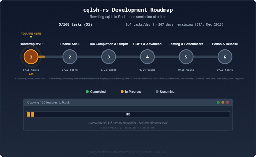
cargo test runs immediately after a change,
failures surface in context, and the next prompt can reference the
actual output. Another reason is just familiarity: the more you use
it, the more you learn to point it at exactly the right problem.
Skills: write your conventions once, use them forever The skills
library was also critical for this project:
/rust-testing – What to test at the unit layer vs. the
integration layer, how to use assert_cmd for CLI
tests, when to reach for insta snapshots
/rust-clippy – Run Clippy with strict
settings and fix everything it complains about
/rust-error-handling – Idiomatic error handling
patterns for this codebase /development-process – The
full loop: review the relevant sub-plan, design tests first,
implement, run tests, update the plan, commit I carried the pattern
directly from coodie. The specific skills are
different (Python vs. Rust), but the idea
is the same. Each skill you write makes every subsequent feature
cheaper to build. Living documents (or, an outdated plan is worse
than no plan) The 19 sub-plans are living documents that are
updated when decisions are made (vs written upfront and then
abandoned, like most docs). When a design decision changes
mid-implementation, the plan changes too. When a task is done, the
checkbox gets ticked. When a new edge case surfaces, it gets added.
This matters more than it might seem. An outdated plan is worse
than no plan because the AI will follow it faithfully…in the wrong
direction. What’s in the box Nothing terribly exotic; there’s: Rust
with Tokio for async. The scylla crate
for the database driver. rustyline for the REPL
and line editing. comfy-table and
owo-colors
for output formatting. testcontainers-rs
for spinning up real Cassandra instances in CI. While the stack
itself might not be exciting, the interesting part is what it takes
to get every CQL type to format exactly like the
Python implementation – right down to float
precision and frozen collection syntax. That’s where
most of the compatibility work lives. Where are we now? Here’s the
same roadmap today:
Phases 1 through 3 are done. The shell works: you can… Connect Run
queries Get formatted output with colors and pagination
Tab-complete keyspace and table names Run 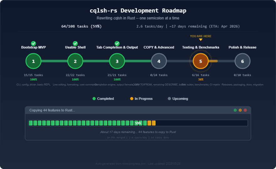
DESCRIBE on
anything Use SOURCE to execute a file Phase 4 –
COPY TO/FROM – is implemented. Phase 5 (testing) is in
progress, with 327 tests and counting. Takeaways Planning
pays (but living documents are a nice touch). A static
plan written at the start and never touched again is a liability. A
plan that gets updated as decisions are made is an asset – and the
primary reason Claude can work effectively across multiple sessions
on a project this size. Skills compound. A good
amount of work is required to find the right skill for the task and
adapt it to the project: the conventions, the patterns, the “this
is how we do it here” info. But once that’s written down, it
becomes easier to implement every feature. The workflow is
never done. The pace of this space is genuinely
disorienting. We now regularly use tools that didn’t even exist six
months ago. This means that what works today might not work in a
month. It’s still writing code, just differently.
(I have a bit of trouble using the word “engineering” here.) Claude
doesn’t replace judgment on architecture, on what actually matters
to users, on “is this the right trade-off?” It removes the friction
between having a clear idea of what you want and that thing
existing. Whether that makes it better or worse probably depends on
the day. Lessons from one project carry over to the
next. The skills pattern from coodie was
carried into cqlsh-rs with a different language and a
different domain. You can start from what you already learned, and
the AI follows the same process docs that you wrote last time.
Things to look forward to One idea that popped up during this: an
--ai-help flag that embeds a small local model to give
offline diagnostics when your CQL query fails. In other words,
building an AI-assisted tool with an AI assistant that will assist
with AI-assisted queries. I’m going to stop thinking about that too
hard. 😉 For the model routing, we’ll probably use
LiteLLM. I heard it’s become quite popular lately. I
had fun. Claude had fun too, probably. I didn’t ask. ScyllaDB Customer Experience Spotlight: Tyler Denton
Welcome to the first installment of a new blog series introducing some of the experts you’re likely to encounter when you work with ScyllaDB. Tyler Denton is a Solutions Architect on the Customer Experience team here at ScyllaDB. He lives in Fort Myers Florida, USA. He’s been at ScyllaDB for about a year, Let’s get to know a little about Tyler… What do you do here at ScyllaDB I’m a Solutions Architect, which is sometimes known as a Sales Engineer or Solutions Engineer. I help customers or prospects review their architectures and find the best place for ScyllaDB to be deployed. Does it make sense, and what’s the most efficient, impactful way to use ScyllaDB in their product or solution? I’m also our field AI subject Subject Matter Expert, so I do a lot with our vector search, a lot with our feature store deployments, agent, state management…things like that. Please share a little about your path to ScyllaDB My first job ever was as a machinist’s mate operating nuclear reactors in the US Navy. That might seem like an odd place to start for somebody who works as a Solutions Architect…but what that taught me was systems. How does the failure of a main steam root valve affect the starboard steam generators? Understanding how complex systems interact and work together taught me a lot about architecture and how to build systems that can survive failure. I started writing software in about the sixth grade and continued doing that, and so I’ve worked at companies like AWS, Couchbase, Rockset (acquired by OpenAI), and that all kind of led me here — where I can focus heavily on bringing large, distributed systems into production and focusing on AI. Tell me about one of the most interesting projects you’ve worked on here One of the most interesting projects I’ve worked on here is an AdTech company that used every feature of our flagship product, ScyllaDB X Cloud. We got to see the major, nearly instantaneous scaling of ScyllaDB. If anybody’s ever used Cassandra or earlier versions of ScyllaDB, you know that wide-table databases can be very hard to scale and can take a long time. Here, we were able to go from 6 nodes to 60 nodes in about 15 minutes, and the throughput and performance we saw from that was absolutely incredible. Watching this develop in real time was very cool and very rewarding. What’s the most impressive ScyllaDB feat you’ve seen a team accomplish Right now, I’m working on bringing a deployment into production where we were displacing another technology. By moving from their existing data model to one supported in ScyllaDB using static maps, we saw a huge cost reduction and a huge performance improvement. They were able to support queries across very complicated data structures in sub-millisecond latency across their entire corpus of data, and they were able to do that because they migrated to ScyllaDB. What do you like to do when you’re not working or on-call When I’m not working my day job, I focus a lot on building my AI knowledge. I do a lot of speaking engagements, development work, and community outreach. And when I’m not doing that, I’m working on my boat. Every now and then I actually get to take it out, but anybody who owns a boat knows that most of the time is spent actually working on it. What’s your top tip for getting the most out of ScyllaDB Follow the instructions. RTFM. Don’t try to be unique. ScyllaDB is designed to solve very specific use cases, and it does that incredibly well. When you try to get creative and build a database within a database, or start doing things ScyllaDB wasn’t designed for, it gets painful really fast, and ScyllaDB will punish you. So just read the manual, follow the best practices, and you’ll have a great time.
ScyllaDB Elastic Scaling in Action [Demo]
Watch along to see how fast ScyllaDB X Cloud scales from 10K to 1M ops/sec and back down again – with single-digit millisecond latency ScyllaDB X Cloud is ScyllaDB’s fully-managed database-as-a-service. It’s a truly elastic database designed to support variable/unpredictable workloads with consistent low latency as well as low costs. We’ve previously blogged about how users can scale out and scale in almost instantly to match actual usage. For example, you can scale all the way from 100K OPS to 2M OPS in just minutes, with consistent single-digit millisecond P99 latency. This means you don’t need to overprovision for the worst-case scenario or suffer the lag traditionally associated with ramping up capacity in response to a sudden surge. In this post, I want to show you how it looks in action: increasing capacity 10X, as well as scaling it back, in minutes. Part 1: Scaling 10X Fast, with Single-Digit Millisecond P99 Latency This first video provides a quick look at how fast ScyllaDB XCloud scales out to increase capacity. It shows you how ScyllaDB’s new tablets architecture lets you scale a cluster to support 10x or more workload capacity in minutes (vs. the usual hours or days). Simulating a massive sales event, we scale a cluster from a moderate 100K ops/sec up to 1M. As we start, the cluster is currently managing a moderate load of 100K ops/sec across three small nodes. Knowing that a surge of 1M ops/sec is imminent, we use the built-in calculator to precisely size our needs. By simply entering the desired read and write throughput and selecting the schema complexity, the system automatically determines the necessary vCPU requirement. In this case, we add three larger nodes to our existing setup. Once the new scaling policy is saved, you can watch the scaling happen as the nodes join and tablets are automatically streamed and rebalanced in parallel. In this demo, the entire scale-out process, including data rebalancing, completed in roughly 23 minutes—all while the cluster remained under load. You’ll see that the new nodes immediately start sharing the responsibility of serving requests even before the rebalancing is fully finished. Finally, we simulate the 10x load jump to 1 million operations per second. You can see that even with mixed instance sizes, ScyllaDB perfectly balances the workload, with the larger nodes serving more requests as expected. Most importantly, despite this massive increase in traffic, the cluster maintains impressive performance. It achieves single-digit millisecond P99 latencies throughout the entire event. Part 2: Achieving Rapid Parallel Scale-Down After Peak Workload This next video demonstrates the process of scaling the ScyllaDB cluster back down to its original size following a simulated high-traffic sales event. You can see how the system handles a drop from 1M ops/sec down to its baseline load. After running at 1M ops/sec for about 20 minutes, our simulated sale event has concluded. That means our load is dropping back to its original 100K ops/sec. Once the load stabilizes and the monitoring overview panel confirms that we are back to 20K writes and 80K reads, we’re ready to scale the cluster back to its original size of 24 vCPUs. To do this, we simply update the scaling policy back to 24 vCPUs. That leaves us with the same three 2x large nodes we had before the simulated sale event started. As the scaling progress begins, we can watch the nodes leave the cluster in real-time. By viewing the monitoring dashboard’s detailed panel, we can see an animation of the tablets streaming from the larger 8x nodes back to the original nodes. Once that’s completed, the cluster is back to its original configuration of three nodes. The scale-down process took about 22 or 23 minutes, which is nearly identical to the time it took to scale up earlier (in the other video). While scaling out has always been fast with tablets, scaling back down used to be a sequential process. Now, starting with version ScyllaDB 2026.1.3, we can scale the cluster in parallel both out and back. That makes it possible to handle a massive workload spike and return to baseline capacity all within about an hour. ScyllaDB Cloud – Free TrialApache Cassandra Performance Tuning: What We Learned
This blog post (tries to) consolidate what we’ve learned from years of tuning Apache Cassandra for performance Here at ScyllaDB, we often run internal and external performance comparisons. Internal testing helps ensure ScyllaDB’s performance advantage, track performance regressions, and maintain compatibility, including catching subtle API semantic-layer changes early. External comparisons are our way to aggregate the performance results for the general public every once in a while. Performance tuning can be a double-edged sword. Overlook one aspect, and you may end up under- or overestimating one’s performance numbers – and that may introduce deep ramifications down the road. While ScyllaDB and Cassandra both share a common API layer and feature set, both systems have fundamentally different architectures. This naturally adds to differences in how each system is tested and tuned. This blog post (tries to) consolidate what we’ve learned from years of tuning Apache Cassandra for performance. We spent a good amount of time hunting down the information we needed. Hopefully, the details described here help others improve their existing Cassandra cluster performance, as well as conduct more meaningful performance comparisons. Side-note: ScyllaDB shares how to reproduce our tests, including references on which settings and parameters we tuned. Check out our Cassandra 4 vs Cassandra 3.11 comparison, my recent talk on how ScyllaDB compares to Cassandra 5, and the comparison between Cassandra vNodes and ScyllaDB tablets as some concrete examples. Overview Perhaps the most relevant Apache Cassandra tuning source publicly available is Amy’s Cassandra 2.1 tuning guide. Despite its 2.1 reference (released in 2014), we find that most of the guidance (or, at least, the high-level concepts) provided there survived the ashes of time, including the array of settings that administrators need to configure by hand. Despite the over-a-decade-long difference, one of Amy’s particular thoughts stands out, and should guide you whenever you’re working with Apache Cassandra tuning:“The inaccuracy of some comments in Cassandra configs is an old tradition, dating back to 2010 or 2011. (…) What you need to know is that a lot of the advice in the config commentary is misleading. Whenever it says “number of cores” or “number of disks” is a good time to be suspicious. (…)” – Excerpt from Amy’s Cassandra 2.1 tuning guide, cassandra.yaml sectionApache Cassandra was originally conceived to run on commodity hardware. It is shipped under the assumption that the end user will configure and tune it for their specific environment. And it also assumes users know what they’re doing. What’s counterintuitive about Apache Cassandra tuning is how small settings can have an outsized impact on performance. Figure 1 perfectly demonstrates this aspect. It shows how both throughput and latencies vary significantly under different GC, compaction, and disk read-ahead settings. Figure 1 – Apache Cassandra 5 performance under different settings One last note before we dive right into tuning specifics: our goal is not to replace Amy’s well-covered, exhaustive guide. Instead, take our words as a complementary reference. We also don’t claim to be experts in the art of Cassandra performance tuning or troubleshooting; rather, we’re practitioners who learned some things (the hard way). Cassandra-Specific Tuning At a minimum, focus your efforts on the following files:
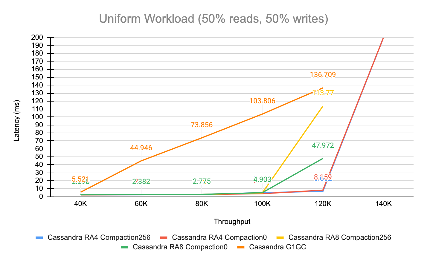
cassandra.yaml
jvm[NN]-server.options
jvm-server.options cassandra.yaml To help
users get started, a stock Apache Cassandra installation ships with
two config files. The first file –
cassandra.yaml – is oriented for users
upgrading from a previous Cassandra release and comes with
backward-compatible settings. The second –
cassandra_latest.yaml – “contains
configuration defaults that enable the latest features of
Cassandra, including improved functionality as well as higher
performance. This version is provided for new users of Cassandra
who want to get the most out of their cluster, and for users
evaluating the technology.” Source:
the Cassandra project. If you spin a fresh
cassandra:5 container or simply initiate your
tuning journey without taking this into consideration, you’ll end
up running your deployment under compatibility mode. The following
command demonstrates how a freshly spun Cassandra 5 container
starts under compatibility mode, rather than enabling its latest
features: root@container:/etc/cassandra# diff cassandra.yaml
cassandra_latest.yaml | sed
's/^>/[cassandra_latest.yaml]/g;s/^</[cassandra.yaml]/g' |
egrep 'compatibility|memtable' | sort [cassandra.yaml]
memtable_allocation_type: heap_buffers [cassandra.yaml]
storage_compatibility_mode: CASSANDRA_4 [cassandra_latest.yaml]
memtable_allocation_type: offheap_objects [cassandra_latest.yaml]
storage_compatibility_mode: NONE It’s beyond the scope of
this write-up to provide an exhaustive list of settings you should
pay attention to when setting up Cassandra. The stock
cassandra.yaml is often irrelevant, and we ended
up simply replacing it with the
cassandra\_latest.yaml instead. If you are
starting a fresh new cluster, we highly recommend you do the same.
However, you probably stream_throughput_outbound_megabits_per_sec option
Both
Cassandra 4.1 and
Cassandra 5.0 docs referenced the
stream_throughput_outbound option Only reading
this
Instaclustr article (or carefully interpreting
cassandra\_latest.yaml) eventually shed some light on the
correct option:
entire_sstable_stream_throughput_outbound. In other
words, 3 distinct settings exist for tuning the previous 3 major
releases of Apache Cassandra – and one of them was incorrectly
documented under the official project’s page. This raises concerns
about the feasibility of upgrading from older releases. Given these
constraints, we highly encourage organizations to conduct a careful
review and full round of testing on their own. This is not an edge
case; others noted similar upgrade problems on the Apache
Cassandra Mailing List. With that in mind, here are some
examples of misleading Cassandra config comments and why upgrades
deserve some extra diligence: CASSANDRA-16315
– Covers the concurrent_compactors setting CASSANDRA-7139
– Describes how that same concurrent_compactors
setting default was production unsafe when introduced CASSANDRA-20692
– Describes how a commitlog correctness issue slipped through to
Cassandra 5 JVM settings Test Kind Garbage Collector Read-ahead
Compaction Throughput P99 Latency Throughput Cassandra RA4
Compaction256 ZGC 4KB 256MB/s 6.662ms 120K/s Cassandra RA4
Compaction0 ZGC 4KB Unthrottled 8.159ms 120K/s Cassandra RA8
Compaction256 ZGC 8KB 256MB/s 4.657ms 100K/s Cassandra RA8
Compaction0 ZGC 8KB Unthrottled 4.903ms 100K/s Cassandra G1GC G1GC
4KB 256MB/s 5.521ms 40K/s Tuning the JVM is the least fun part of
operating a Cassandra cluster. It can be a journey on its own,
really. The good news is that Cassandra 5 includes support for
JDK17, and users may now opt-in for using ZGC rather
than the decades-long G1 garbage collector. Unless you
are a Java expert and know exactly what you are doing, this
theLastPickle article is perhaps your best resource for tuning
Cassandra’s JVM. You could read that and call it a day. Still, here
are some details on what we’ve discovered along the way, since the
DataStax (now IBM)
Tuning Java resources page only advises under a remark
of adjusting “settings gradually and test each incremental
change”: We’ve consistently measured lower latencies and
higher throughput using ZGC under a handful of
different scenarios. Although we’ve seen some users reporting good
G1 performance results, this doesn’t align with what
we’ve experimented with in practice. Remember that Cassandra relies
on both off-heap as well as on-heap memory. The heap size will
depend on how much RAM your setup has. Since we primarily test on
128GB RAM machines, we found that allocating beyond 32G would be
wasteful.
theLastPickle‘s article mentioned earlier makes a good point
about compressed OOPs, though we believe this should be relevant
for RAM constrained systems. We didn’t observe any noticeable
benefits/disadvantages from having 31G/32G in our
results. Most of the JVM settings will sit under the
jvm17-server.options file (if you’re using
JDK17). However, there is yet another file
(jvm-server.options, note there’s no Java
version) that you should also edit. Apparently Cassandra has some
built-in scriptology in cassandra.in.sh that
looks up the latter and inherits options from it. Then, if your
heap settings (-Xmx & -Xms) are unset, it
will automatically define it for you: ################# #
HEAP SETTINGS # ################# # Heap size is automatically
calculated by cassandra-env based on this # formula: max(min(1/2
ram, 1024MB), min(1/4 ram, 8GB)) # That is: # - calculate 1/2 ram
and cap to 1024MB # - calculate 1/4 ram and cap to 8192MB # - pick
the max # # For production use you may wish to adjust this for your
environment. # If that's the case, uncomment the -Xmx and Xms
options below to override the # automatic calculation of JVM heap
memory. # # It is recommended to set min (-Xms) and max (-Xmx) heap
sizes to # the same value to avoid stop-the-world GC pauses during
resize, and # so that we can lock the heap in memory on startup to
prevent any # of it from being swapped out. #-Xms4G #-Xmx4G
Therefore, uncomment and override the two lines above for your
environment. After you are done, you may want to circle back to the
cassandra.yaml file because there are some
settings that influence your heap allocation. For example:
networking_cache_size file_cache_size
memtable_offheap_space
repair_session_space among others… If you feel like
Cassandra is choking and the system is not under heap pressure,
then playing with these settings is probably your next step. Sadly,
this is where things become trial-and-error, and even more time
consuming. (Though, in Cassandra’s defense, tuning most of these
parameters is workload specific). About Cassandra Caching
Apache Cassandra ships two caching-related settings:
row_cache_size and key_cache_size You
should almost never enable either of these settings
(0GiB means these are disabled). The only exception is
when your workload has a (VERY) high cache hit ratio and is
relatively static. The table below shows how both Row & Key caches
have a negative performance impact in Cassandra during a scale-out:
Kind Step
Throughput Retries
Cassandra 5.0 – Page Cache 3 > 6 nodes 56K ops/sec 2010
Cassandra 5.0 – Page Cache 6 > 9 nodes 112K ops/sec 0
Cassandra 5.0 – Row & Key Cache 3 > 6 nodes 56K ops/sec 5004
Cassandra 5.0 – Row & Key Cache 6 > 9 nodes 112K ops/sec
8779 Likewise, Figure 2 shows how throughput varies significantly
under a fully cached workload:
Figure 2 – Cassandra Row Cache vs OS Page Cache
performance (speedup falls between 1.14x to 1.5x)
An old
DataStax (IBM) documentation page strongly discourages its use,
noting that users should prefer using the OS page cache instead:
Note: Utilizing the appropriate OS
page cache will result in better performance than using row
caching. Counterintuitively, DataStax (IBM) later recommends
enabling the Row Cache when the number of reads dominate compared
to writes: Tip: Enable a row cache
only when the number of reads is much bigger (rule of thumb is 95%)
than the number of writes. Consider using the operating system page
cache instead of the row cache, because writes to a partition
invalidate the whole partition in the cache. OS Tuning
Operating system tuning for Cassandra shares many similarities with
other databases. Preventing swapping, tuning the kernel via
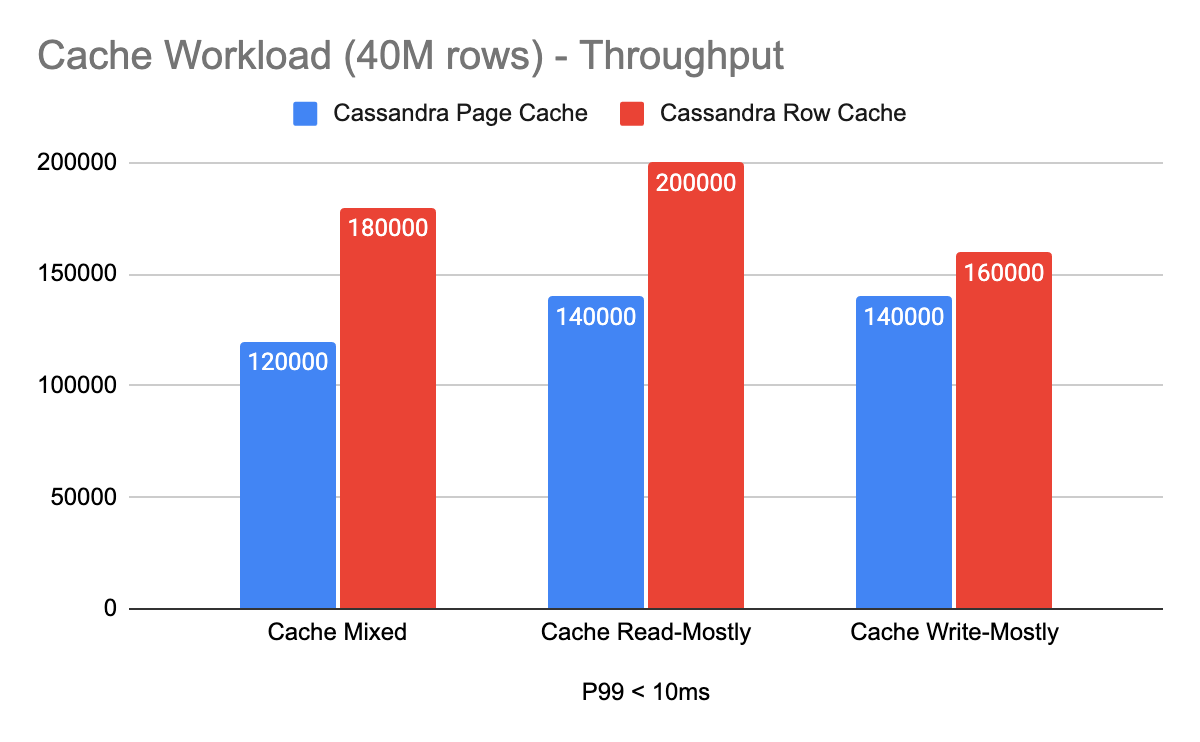
sysctl, setting disk read_ahead_kb
settings, configuring user limits and enabling Transparent
HugePages are the primary settings we touch when deploying
Cassandra. This is (undoubtedly) a non-exhaustive list, although it
should cover the strategies seen across most production Cassandra
deployments in practice. Depending on your setup, you may want to
further check: your
clocksource – particularly under Xen hypervisors; whether
cpupower supports setting the CPU scaling governor to
“performance” mode; experimenting with jemalloc;
configuring SMP IRQ
Affinity; and pinning Cassandra to specific CPUs via taskset(1).
Disks We primarily store Cassandra related files (including its
related logs) on locally-attached NVMe disks, as commonly found
within cloud hyperscalers. If there’s more than one attached disk
to the VM, we combine them into a RAID-0 array using
mdadm. In addition, we use XFS as the
backing filesystem, particularly as it’s the same we use for
ScyllaDB. We also set only one-hit merges, limit
read_ahead_kb to just 4kB, and disable
the IO scheduler (if any): MD_NAME=nvme1n1 sudo sh -c "echo 1
> /sys/block/$MD_NAME/queue/nomerges" sudo sh -c "echo 4 >
/sys/block/$MD_NAME/queue/read_ahead_kb" sudo sh -c "echo none >
/sys/block/$MD_NAME/queue/scheduler" Some important remarks:
the scheduler command may “fail” in modern Cloud
instances (and that’s fine); when using mdadm, tune
each block device individually backing the RAID device;
read_ahead_kb is a workload dependent setting. We
often test small partition lookups, but workloads with larger
wide-rows may benefit from increasing that setting. Memory We don’t
configure swapping at all to keep matters simple. The rationale is
that Cassandra already benefits from the OS page cache, and we
leave over half of the server’s RAM just for it. During our tests,
we also observed that enabling Transparent Huge pages,
especially with ZGC, contributed positively to
Cassandra’s performance. Although the improvement wasn’t
remarkable, we observed positive results similar to what both
Amy and
Netflix reported. The provided links already go in-depth on how
to enable THP, as well as how to configure Cassandra
to benefit from it. Keep in mind, however, that we recommend you
set the -XX:+AlwaysPreTouch JVM option regardless of
whether THP is enabled or not. That’s because it’s
known to improve overall JVM runtime performance at the expense of
increased JVM startup times. Kernel and User limits Put simply, you
don’t want Cassandra to be limited on either networking, memory
allocation, or the number of files it can open. We set
sysctl.conf.d/99-cassandra.conf to the following
values: net.ipv4.tcp_keepalive_time=60
net.ipv4.tcp_keepalive_probes=3 net.ipv4.tcp_keepalive_intvl=10
net.core.rmem_default=16777216 net.core.wmem_default=16777216
net.core.optmem_max=40960 vm.max_map_count = 1048575
net.ipv4.tcp_rmem = 4096 87380 16777216 net.ipv4.tcp_wmem = 4096
65536 16777216 net.core.rmem_max = 16777216 net.core.wmem_max =
16777216 net.core.netdev_max_backlog = 2500 net.core.somaxconn =
65000 net.ipv4.tcp_ecn = 0 net.ipv4.tcp_window_scaling = 1
net.ipv4.ip_local_port_range = 10000 65535 net.ipv4.tcp_syncookies
= 0 net.ipv4.tcp_timestamps = 0 net.ipv4.tcp_sack = 0
net.ipv4.tcp_fack = 1 net.ipv4.tcp_dsack = 1
net.ipv4.tcp_orphan_retries = 1 vm.dirty_background_bytes =
10485760 vm.dirty_bytes = 1073741824 vm.zone_reclaim_mode = 0
fs.file-max = 1073741824 vm.max_map_count = 1073741824
Lastly, the user running Cassandra must be allowed to allocate
enough resources for the process to run. As our VMs are
short-lived, we enable unlimited limits.conf
consumption to all users: * - nofile 1000000 * - memlock
unlimited * - fsize unlimited * - data unlimited * - rss unlimited
* - stack unlimited * - cpu unlimited * - nproc unlimited * - as
unlimited * - locks unlimited * - sigpending unlimited * - msgqueue
unlimited Parting Thoughts As demonstrated, Apache Cassandra
performance tuning is far from a one-size-fits-all solution. The
settings described throughout this article represent what worked
for our specific hardware setups and workload profiles. If your
deployment spans different hardware, many of the values presented
here will likely need to be revisited. This brings us to (perhaps)
the most underappreciated cost in Cassandra operations: dependency.
That is, every tuning decision is implicitly a contract with the
underlying hardware. Adding more disks, increasing CPU/RAM,
changing workloads are some overlooked aspects that will require
entirely new tuning cycles and re-evaluating your previous
decisions. ScyllaDB was designed with this problem in mind. Its
shard-per-core architecture and self-tuning capabilities
automatically adapt to the underlying hardware, eliminating much of
the manual iteration and tuning described here. There’s no JVM at
all, and most of the OS heavy lifting is carried out for you via an
automated script shipped alongside the core database. If Cassandra
performance has been a bottleneck, you’re concerned about the
recent IBM acquisition, or you’ve simply spent too much time
fighting tuning instead of building – give ScyllaDB a try. And if
you want to have a technical
discussion about your use case, let us know. “Key-Value” is Misleading. Access Patterns are Key.
Access patterns determine your data model, your I/O costs, and which database is the best fit for your workload I’ve been part of enough key-value database evaluations to recognize the pattern. When the conversation starts with benchmarks, the evaluation inevitably ends with regret. The benchmark answers “which is faster?” It doesn’t tell you which model fits how your application actually reads and writes data – and that’s what matters. Every data modeling decision should begin with access patterns, regardless of the technology on the table. What does your application read? At what granularity? What does it write? How often? How large? Let those answers drive the data model, then pick the technology. Flip that order and you pay for it. A fast database like ScyllaDB amplifies schema decisions: good models perform well, bad ones break faster. Edgar Codd invented First Normal Form (1NF) in 1970 to save disk space, but a terabyte of NVMe now costs about the same as lunch. So, even though the rule outlasted the constraint that justified it, we are still teaching it. That’s partly why so many teams expect to normalize their data with ScyllaDB the way they would a relational schema. But if they don’t get the order right (access patterns> data model> technology), they won’t get the performance that the engine was built to deliver. A lot of the confusion comes down to terminology. “Key-value” is one of the most overloaded labels in the database industry. We use it to describe both: A system that maps a string to an opaque blob A system that maps a partition key plus a clustering key to typed, individually addressable columns with partial-update semantics. Lumping these together hides the architectural decisions that determine your I/O patterns and your infrastructure costs. “Key-value” is often used to describe three very different data models. They differ in capability and in how deeply you can address your data. Pick the wrong one for your access patterns and you pay for it in I/O overhead, infrastructure cost, and write throughput. ScyllaDB can operate across multiple levels of this hierarchy. The one you select influences your I/O patterns, your update costs, and your infrastructure spend. Key-Value vs Wide-Column: Four Levels of Access Pattern Depth Instead of looking at feature lists, it’s better to compare these models by access pattern depth: at what level can you address, read, and write your data? Level 1: Key level. One key maps to one value. The value is opaque. The database has no knowledge of what is inside it. You get it and you put it in. This is K-V, the model behind most caching layers and session stores. Redis is the canonical example. The ceiling is the value boundary – you can replace it, you cannot address inside it. Level 2: Row level. A primary key maps to a set of named bins. Each bin holds a schemaless value. You can address individual bins by name, you can project specific bins in a read, and you can also update bins independently. This is K-V Wide Table, one key, multiple named fields, no schema enforcement on values. This model adds meaningful structure over K-V without requiring upfront schema design. Aerospike is the canonical example here. The ceiling is the bin boundary – you can update a bin, but you cannot address inside one. Level 3: Column level. A partition key combined with a clustering key addresses a row. Each column in that row is individually typed. The database understands the type of every value it stores. This is KKV Wide Table, the two-key model is what puts the second K in KKV. Typed columns enable the database to make smarter decisions about storage layout, compression, and update semantics. Cassandra reaches this level. The ceiling is the column boundary – typed and addressable, but complex values inside a column must be declared frozen. In other words, the entire value is serialized as a single blob that the engine cannot see into. Level 4: Within-column level. This is a key differentiator for KKV Wide Table. The engine starts working at a granularity that the other models can’t reach. A KKV Wide Table column can hold a collection: a map, a set, a list, a user-defined type, or nested combinations of these. Whether the database can address what’s inside that collection determines your actual access pattern depth. A frozen collection is serialized as a single blob. The engine stores it, retrieves it, and replaces it, but cannot see inside it. An unfrozen collection is stored element by element. Each entry is individually addressable. That distinction is the central architectural argument at this level. Cassandra touches this level but can’t reliably live here. Unfrozen collections exist in Cassandra, but tombstone accumulation makes them a liability in production. In ScyllaDB, Level 4 becomes practical. With an unfrozen collection, ScyllaDB stores each element individually. Whether you add an entry to a map, append to a list, or remove an element from a set – no read is required first and the database operates at element level. With a frozen collection, ScyllaDB serializes the entire value as a single cell. The engine can’t address inside it. For whole-value access patterns, that’s not a limitation, it’s an optimization. With this: There’s no per-element metadata. Reads pull one contiguous cell. Writes replace one contiguous cell. ScyllaDB’s UDT performance benchmarks show frozen collections outperforming unfrozen ones by up to 228% on write throughput and 162% on read throughput for 50-field UDTs. For the right access pattern, frozen is the faster choice. Don’t focus on frozen vs unfrozen; look at access pattern first and the right tool should follow from there. Figure: Frozen vs. unfrozen UDT, 50-field profile accessed as a whole. Frozen write throughput 228% higher, read throughput 162% higher. One cell write vs. 50-element writes plus 50 metadata records. The problem isn’t that it’s frozen; the access pattern mismatch is what’s causing the performance difference. An engineer who needs element-level updates and chooses frozen UDTs has, for those columns, given back Level 4 access. The operation degrades to read-modify-write: read the entire value, apply the change in memory, write it back as a whole. That is the same pattern a K-V Wide Table bin requires. The technology supports Level 4, but the schema choice has opted out of it. Figure: Four levels of access pattern depth. K-V gives key-level access. K-V Wide Table adds bin projection. KKV Wide Table adds typed columns and, with unfrozen collections, element-level access. Frozen collections are a performance optimization for whole-value access patterns, not a fallback. The opposite mistake is also a problem. An engineer who uses large unfrozen collections for values they always access as a whole pays per-element TTL and timestamp metadata on every element in the collection – at compaction time, continuously. A map with 10K entries carries 10K individual metadata records. That overhead snowballs over time. Choose frozen collections when you access the value as a whole. Choose small unfrozen collections when you need element-level updates. Large unfrozen collections are their own design smell, regardless of access pattern. Figure: Read granularity, requesting one field from a 30-field record. K-V reads the entire blob. K-V Wide Table reads the entire record and returns one bin. KKV Wide Table reads only the requested column, leaving 29 columns untouched on disk. How Access Pattern Depth Meets Memory: Three Scenarios The relationship between your dataset size and available memory determines which architecture is working with its strengths and which one is working against them. Figure: Data model behavior across memory scenarios, relative I/O and cost overhead for K-V, K-V Wide Table, and KKV Wide Table as dataset size moves from fits-in-RAM through keys-only-in-RAM to neither-fits-in-RAM. Scenario 1: Everything Fits in Memory When the entire dataset lives in RAM, a memory-resident hash index is fast. Point lookups are a hash computation and a pointer dereference. This is where K-V and K-V Wide Table architectures shine for read latency. But “what’s fast?” and “what’s cost-effective?” are different questions. If your dataset is 2 TB, you are paying for 2 TB of RAM across your cluster. An architecture designed around SSDs with efficient memory-resident metadata can deliver reads in the low hundreds of microseconds while your data lives on storage that costs a fraction of RAM per gigabyte. Although the access pattern performance difference on reads may be negligible, the infrastructure cost difference is not. Figure: Storage cost at scale, all-RAM vs NVMe SSD across dataset sizes from 0.5 TB to 32 TB. DDR5 ECC at ~$8/GB vs NVMe SSD at ~$0.10/GB. The gap compounds quickly past 1 TB. This is also the scenario where honesty matters. If your access pattern is truly “put blob, get blob” on ephemeral data with simple lookups, a K-V store is the right tool. The operational simplicity is a genuine advantage. There are fewer moving parts and fewer things to misconfigure. If your values are small and your queries never need to reach inside them, a K-V store will serve you well and be easy to operate. Scenario 2: Keys Fit in Memory, Values Do Not This is what K-V Wide Table architectures market as their sweet spot. Here, you have a primary index in memory, records on SSD, and fast key lookups that pull values from disk. For simple reads, bin projection works well here. Request three specific bins, get three bins back. You are not forced to read the entire record on every read. The problem surfaces at Level 4. Assume one bin holds a serialized map of user preferences and you need to update a single entry in that map. In this case, the system must: Read the entire bin from disk Deserialize the collection structure in memory Apply the modification Serialize the updated structure Write the entire bin back. That is a read-modify-write cycle on every collection update, regardless of how small the change is. The K-V Wide Table model has no path to Level 4 access. The bin is the floor. A KKV Wide Table model with unfrozen collections handles the same update without a read. The new map entry goes directly to the write-ahead log and the in-memory table. There’s no deserialization or full-bin read. The merge with existing data happens during compaction, as a background operation that does not block the write path. Compression: typed columns vs. schemaless bins. K-V Wide Table bins are schemaless. Within an SSTable block, different records interleave bin data without type information. That limits what a compressor can do across records. A KKV Wide Table stores typed column data within the same partition contiguously in SSTable blocks. For example, ScyllaDB writes all values for the event_ts column across rows in a partition together. Because those values share the same type, a dictionary-based compressor like zstd has much more to work with. This is not columnar storage in the analytics sense. ScyllaDB is an LSM-tree row-based engine at the partition level, not Parquet. The compression benefit comes from typed column homogeneity within SSTable blocks rather than a columnar storage layout. Frozen vs. unfrozen compression tradeoffs. Frozen UDTs compress well for a specific reason. A frozen UDT is a single cell with a consistent serialized layout. The same 50-field structure appears as the same byte sequence across records, which dictionary compression handles efficiently. Unfrozen collections are a different story. Each element carries its own TTL and timestamp metadata. ScyllaDB groups column values within SSTable blocks, which helps the element values themselves compress, but the metadata overhead scales with collection cardinality. For small unfrozen collections, it’s negligible. For large unfrozen collections, it can negate a meaningful portion of the compression gain. The compression advantage of typed columns applies most cleanly to simple typed columns and small unfrozen collections. Figure: K-V Wide Table SSTable blocks mix types across schemaless bins, limiting compression. KKV Wide Table SSTable blocks group typed column data within partitions. Frozen UDTs compress well as consistent serialized blobs. Unfrozen collections carry per-element metadata that can offset compression gains at high cardinality. Data locality. In a shard-per-core architecture (e.g., ScyllaDB’s), all columns within a partition live on the same CPU core. A read that touches three columns in a single partition involves zero cross-core coordination. This avoids locking and message passing between threads. This data locality might not be significant at low throughput. However, it matters a lot at hundreds of thousands of operations per second. Scenario 3: Neither Keys Nor Values Fit in Memory This is where memory-dependent index architectures hit a wall. If your architecture puts the primary index in RAM and your keyspace outgrows available memory, you are either: Adding nodes to hold the index, or Paging index entries to disk, which adds a disk read in front of every data read An architecture built for disk-resident data from the start does not have this problem. ScyllaDB (and to a degree Cassandra) uses Bloom filters to determine probabilistically whether a partition exists in a given SSTable without loading a full index into memory. Partition index summaries provide efficient lookup with a small, fixed memory footprint regardless of key count. And compaction strategies manage on-disk data organization to keep read amplification bounded. This is all strategic design for an architecture that assumes data will not fit in memory. Don’t just think about whether a system can handle disk-resident data; consider whether it was designed for it. The Update Path: Where Access Depth Becomes I/O Pattern Most evaluations obsess over reads. However, the update path is where access pattern depth differences tend to surface at scale. Consider updating a single element in a collection, one value in a map with 500 entries. In a K-V Wide Table architecture, collection updates require a full read-modify-write cycle: read the entire bin from disk, deserialize the collection structure in memory, apply the modification, serialize the updated structure, then write the entire bin back. Under concurrent updates to the same record, this becomes a serialization bottleneck. Under write-heavy workloads, write throughput is gated by read throughput. Figure: K-V Wide Table collection update path. A single-element update requires reading, deserializing, modifying, serializing, and rewriting the entire bin. In a KKV Wide Table architecture with unfrozen collections, the same update works like this: write the new value for that map entry directly to the memtable. This avoids the read, the deserialization, and the serialization. The entry lands in the write-ahead log and the in-memory table. The merge with existing data happens during compaction, as a background operation. Figure: KKV Wide Table update path with unfrozen collection. The write goes directly to WAL and memtable. No read required. Compaction merges data in the background. This is where access pattern honesty matters most. The append-only unfrozen update is fast for element-level changes to bounded collections. When your access pattern is whole-value, you write the entire UDT atomically and read it back as a unit. Here, frozen is the right choice. There is no read penalty and no per-element overhead. The ScyllaDB UDT benchmark shows 228% write throughput improvement for frozen UDTs in exactly this scenario: a 50-field UDT accessed and written as a whole. The frozen cell is one write operation. The equivalent unfrozen collection is 50 element writes plus 50 metadata records. The difference at 1,000 operations per second is negligible. But at 100,000 operations per second, with large collections and concurrent writes, the wrong frozen/unfrozen choice becomes the bottleneck in either direction. Figure: Write latency vs. collection size for a single-entry update. K-V Wide Table read-modify-write latency grows linearly with the number of entries in the collection. KKV Wide Table unfrozen update latency stays flat, the write goes to the WAL and memtable regardless of collection size. Figure: Single-element update latency vs. collection size, illustrating how wasted I/O grows with collection size for read-modify-write architectures, while direct-write latency remains constant. Choosing Honestly: Key-Value, K-V Wide Table, or KKV Wide Table These three models exist because different access patterns have different requirements. K-V is the right model for caching, session storage, and any workload where the access pattern is “put blob, get blob.” Its simplicity is a real advantage because you end up with fewer moving parts and fewer things to misconfigure. If your values are small and your queries never need to reach inside them, a K-V store will serve you well and be easy to operate. K-V Wide Table adds meaningful capability for workloads that need to address individual fields without upfront schema design. It’s a pragmatic choice for moderate-scale applications where operational simplicity matters, bin-level read projection is sufficient, and collection updates are infrequent or small. It sits at Level 2–3 access depth and does that job well. KKV Wide Table earns its complexity when your access patterns require Level 3 or 4 depth: frequent updates to large collections, datasets that will outgrow available memory, workloads where typed column compression meaningfully reduces storage cost, or write-heavy workloads that cannot afford read-modify-write on every collection update. The richer data model requires upfront schema design and demands that you get frozen versus unfrozen semantics right. Don’t rely on your intuition; choose strategically, based on your actual access pattern: Use frozen when you always read or write the whole value. A 50-field profile UDT that you always write and read back as a unit is a frozen candidate. The performance data supports it. Use small unfrozen collections when you need element-level updates. Append to a list. Update one key in a map. This is what unfrozen exists for. Use large unfrozen collections only if your access pattern is genuinely element-granular and your collection cardinality stays bounded. Per-element metadata overhead compounds. It affects both compaction cost and compression ratios. Figure: Decision flow for choosing a data model based on required access pattern depth. Don’t focus on which model is “best.” Think about which model best matches the access patterns your workload will experience in production. Start with the access patterns. Let the data model follow. Then pick the technology that supports that model at the depth you need. Get that order right and the database works with you. Get it wrong, and you spend your time working around it. *** If your use case requires low latencies at scale, and you’re frustrated with fighting your current database, ScyllaDB Cloud might be worth a look. Find me on LinkedIn – I’m always happy to talk data models.
What’s new in Cassandra® 6? A roundup of features for users and operators
Apache Cassandra 6 is shaping up to be significant release as some of its biggest changes affect the core behavior of the database:
- How metadata is coordinated
- How Cassandra is moving toward broader transaction support via Accord protocol
- How repair is scheduled, and
- How operators inspect and manage the system.
Let’s focus on a few changes that stand out:
- Accord transactions
- Transactional Cluster Metadata (TCM)
- Automated repair
- Constraints framework
- Zstandard dictionary compression, and
- Cursor-based compaction improvements.
Taken together, these changes point to a version of Cassandra that is becoming more structured internally and easier to operate.
Accord transactions for ACID guaranteesAccord is a general-purpose transaction framework that uses a leaderless consensus protocol to have highly available transactions and is used in Cassandra 6. The goal is broader transactional support across multiple keys, with strict serializable isolation and without a central bottleneck.
This matters because multi-key consistency is hard to handle cleanly in application code. Once a workflow spans more than one partition, the application often ends up doing coordination work that really belongs in the database.
Accord enables ACID behavior on transactional tables, which lets developers coordinate multi-step, multi-partition changes with stronger correctness guarantees, reducing the amount of custom consistency logic they have to build in the application.
Including multi-partition, conditional work has historically been difficult to express cleanly in Cassandra. For operators, it signals that transactions are becoming a more important part of the platform and something to watch closely as Cassandra continues to mature.
Read our deep dive on Accord transactions here.
Transactional Cluster Metadata (TCM)TCM changes how Cassandra coordinates cluster-wide metadata. TCM introduces a Cluster Metadata Service that keeps an ordered log of metadata changes and makes those changes visible in a more consistent, coordinated way. That includes things like membership, token ownership, and schema state.
This was introduced because Cassandra’s older model depended heavily on eventual consistency and the Gossip Protocol to spread metadata changes across the cluster. TCM is meant to make those changes more explicit, more ordered, and easier to reason about.
For operators, this is one of the biggest architectural shifts in Cassandra 6. It does not mean Gossip Protocol disappears everywhere, but it does mean Cassandra is moving away from Gossip as the primary way cluster membership, schema, and data placement changes are coordinated and made visible. For users, the result should be more predictable schema and topology operations.
Automated repair orchestrationAutomated repair brings repair orchestration into Cassandra itself. Repair is the mechanism Cassandra uses to reconcile replicas over time so they stay consistent, and the goal is to make repair scheduling and coordination a built-in database service rather than something operators must orchestrate with external tools.
This was introduced because repair is essential, but historically it has placed a real burden on operators. Teams have had to build their own schedules, decide how to run repair safely, and keep it consistent over time.
For operators, automated repair could be one of the most practical changes in the release. It reduces manual coordination, supports full and incremental repair, adds useful safeguards, and makes repair easier to treat as a normal part of cluster maintenance—just like it has happened with major compactions with Unified Compaction Strategy in Cassandra 5. For users, it means a better chance that maintenance happens regularly and with fewer gaps.
At NetApp Instaclustr, our expert TechOps team already orchestrates laborious tasks like repair for our Apache Cassandra customers, ensuring their clusters stay online. Our platform handles the complexity so you can get up and running fast.
Constraints framework for data validationThe constraints framework lets Cassandra enforce more targeted
validation rules as part of the table schema. It enforces them at
write time instead of relying entirely on application code to
reject invalid data. Some examples of constraints include: Scalar
(>, <, >=,
<=), LENGTH(),
OCTET_LENGTH(), NOT NULL,
JSON(), REGEXP().
A simple example of an in-line constraint:
CREATE TABLE users ( username text PRIMARY KEY, age int CHECK age >= 0 and age < 120 );
This was introduced because Cassandra already had some broad limits, but they were not very granular or expressive. The constraints framework gives teams a more precise way to protect the shape of their data and guard against bad writes from misconfigured clients.
Operators gain more control and better predictability around what gets written into the cluster. For developers, it means some validation can move closer to the schema instead of being duplicated across every service.
Zstd dictionary compressionZstandard, or Zstd, dictionary compression extends SSTable compression by letting Cassandra use trained Zstd dictionaries for repetitive data patterns. Instead of relying only on generic compression, it can use a dictionary built from representative data to improve results.
This was introduced to primarily improve compression ratio while keeping the design manageable in production. It is recommended to use minimal dictionaries and only adopt new ones when they’re noticeably better.
This makes compression more configurable and more visible for operators. It adds training workflows, dictionary lifecycle management, and observability into dictionary size and cached dictionary memory usage. For users, the main benefit is better storage efficiency, because data with strong repeating patterns can compress better, leading to potential performance gains.
You can read more about the constraints framework and Zstd dictionary compression in our article detailing recent CEPs.
Cursor-based compaction improvementsCursor-based compaction is a new low-allocation compaction path in Cassandra 6 that processes SSTable data in a more streaming-oriented way, using reusable cursor-like readers and writers instead of constantly creating large numbers of temporary in-memory objects. In practical terms, it is designed to reduce heap allocation and garbage collection overhead during compaction.
Compaction is one of Cassandra’s most important background processes, and when it becomes cheaper and more efficient, nodes can spend less time fighting garbage collection and less heap on temporary work. For operators, that can mean smoother performance and better efficiency on large datasets. For developers, it is mostly an under-the-hood improvement, but one that can help clusters behave more consistently under load.
Conclusion: A more manageable databaseWhat stands out about Cassandra 6 is that many of its biggest changes are not isolated features. They reshape core parts of how Cassandra behaves and how it is operated.
Accord introduces a broader transactional model. TCM changes how metadata is coordinated. Automated repair brings a core maintenance task into the database. Constraints make schemas more defensive. Zstd dictionary compression improves how Cassandra approaches storage efficiency, and cursor-based compaction makes the system easier to run.
Taken together, Cassandra 6 focused on making the database more deliberate internally and more manageable operationally.
Stay tuned for a preview release of Cassandra 6 on the Instaclustr Platform!
Ready to get started?If you want to experience the power of Apache Cassandra without the operational headache, we have you covered. If you are an existing customer and would like to try Cassandra 5 before 6.0 is released, you can spin up a cluster today. If you don’t have an account yet, sign up for a free trial and experience the latest generation of Apache Cassandra on the Instaclustr Managed Platform.
Read all our technical documentation here.
Discover the 10 rules you need to know when managing Apache Cassandra.
If you are using a relational database and are interested in vector search, check out this blog on support for pgvector, which is available as an add-on for Instaclustr for PostgreSQL services.
The post What’s new in Cassandra® 6? A roundup of features for users and operators appeared first on Instaclustr.
Introducing ScyllaDB Agent Skills
A new set of best practices and usage patterns for AI agents working with ScyllaDB Cloud clusters Today we’re releasing a curated set of best practices and usage patterns for AI agents working with ScyllaDB Cloud clusters. If you just want to grab the skills and go build, here you go:npx skills add
scylladb/agent-skills If you want to understand why these
skills are useful and what problems they solve, read on. ** You may
have noticed a short warning at the bottom of many AI applications:
“AI can make mistakes. Double-check the output.” Or something along
those lines. This is also true when it comes to working with
databases. We’ve seen agents reach for the wrong driver, fail to
connect to ScyllaDB Cloud, generate schemas that fit a relational
database but not NoSQL, and produce queries that technically
execute but perform poorly at scale.
For more on agents getting things wrong, see this video…These problems can all be minimized by using agent skills. What are Agent Skills? Agent Skills are markdown files that give your AI agent best practices and domain-specific knowledge. They follow the standard format and help your agent reduce hallucinations. They are also essential to give the agent up-to-date information. Since LLM training data doesn’t include real-time updates by default, these skills help bridge that gap. A specialized skill helps make the agent’s behavior more consistent and predictable. Available ScyllaDB Skills The ScyllaDB Agent Skills cover three distinct areas: scylladb-cloud-setup: Guides agents through the full connection flow: retrieving cluster credentials from the Cloud Console, selecting the correct shard-aware driver for the user’s language, configuring DC-aware load balancing with the right datacenter name, and verifying the connection. scylladb-data-modeling: Encodes query-first design methodology, partition key and clustering column patterns, anti-patterns (
ALLOW FILTERING, hot partitions,
unbounded partition growth), time-series bucketing, and guidance on
when to use secondary indexes versus denormalized tables. The goal
is to create schemas and queries that hold up under production load
(just returning correct results in development is not sufficient).
scylladb-vector-search: Covers vector index
creation, ANN queries, filtering strategies (global vs. local
indexes and when each applies), quantization, and driver
configuration. You can install all three at once, or pick only what
your project needs. Each skill loads on demand when a relevant task
comes up, they don’t interfere with each other. Let’s look at the
main areas where AI systems get ScyllaDB wrong. Shard-aware drivers
ScyllaDB has its own family of shard-aware drivers for Python,
Java, Go, Rust, C++, and
more. Agents sometimes decide to download the wrong driver.
While it may appear to work, unofficial drivers bypass ScyllaDB’s
shard-aware routing and degrade performance. In other cases, agents
may hallucinate non-existent drivers. Besides making it impossible
to connect to the ScyllaDB cluster, this also introduces a security
risk: you may install a fake package designed to trick the AI (this
is called slopsquatting).
Connecting to ScyllaDB Cloud Connecting to ScyllaDB Cloud requires
DC-aware load balancing configured with the exact datacenter name
(e.g. AWS_US_EAST_1) from your cluster. If your agent
gets that wrong, the driver will fail to connect. Data modeling
ScyllaDB’s data model requires you to have a query-first approach.
You design tables around your access patterns, not your entities.
Agents tend to be trained more heavily on SQL and relational
databases than on NoSQL systems such as ScyllaDB. That means they
are more likely to generate an entity-first schema, then use
ALLOW FILTERING to force queries. This can result in
suboptimal performance when using ScyllaDB. Vector Search Vector
search on ScyllaDB is powerful but specific. There are global and
local vector indexes with different filtering semantics and
performance considerations. There’s an ANN OF
operator, and quantization options that matter at scale. Choosing
the wrong index type for a filtered query can hurt performance.
Getting started Install all skills using the Vercel Skills CLI
(requires Node.js): npx skills add
scylladb/agent-skills Or install a specific skill: npx
skills add scylladb/agent-skills --skill
scylladb-data-modeling You can also install manually by
cloning the GitHub repository
and copying the skill folders into your agent’s skills directory:
Agent Skills directory Claude Code ~/.claude/skills/
Cursor ~/.cursor/skills/ OpenAI Codex
~/.codex/skills/ OpenCode
~/.config/opencode/skills/ The skills follow the
Agent Skills open standard
and work with any agent that supports it, including Claude Code,
Cursor, Codex, and GitHub Copilot. Native Claude Code and Cursor
plugins are coming soon. We recommend installing all three skills
in any project that uses ScyllaDB. You get full coverage of the
areas where agents most commonly go wrong, with no overhead when
those skills aren’t relevant to the current task. As of now, the
skills cover the CQL interface; Alternator (DynamoDB
API) is not yet included. Feedback is welcome. Create an
issue on GitHub! New Research on Cloud Database Trends: Technical Risks, Cost Pressures, and Migration Triggers
Good enough until it isn’t: the database complacency trap A database is like a water heater. When all is well, it just does its job in the background. You don’t fantasize about replacing it or envy the one your friend just got. Really, you don’t even think about it — until something goes awry. But new research reveals a key difference: With databases, the problems don’t blindside you. Some 38% of technology leaders worry that their current database won’t meet their needs in the near future. However, they aren’t acting on it. They wait until some compelling event (e.g., a production incident, usage spike, budget cut, or cloud strategy pivot) pushes the database to the top of the priority list. That’s just one of the interesting findings from the Futurum Group’s latest research study, commissioned by ScyllaDB, which explores the latest trends in cloud database cost pressures, performance risks, and migration motivations. Respondents include technical decision-makers who shape cloud database strategy as well as team members directly responsible for the database. Guy Currier, Futurum Group Chief Analyst, summarizes the findings this way: “Those technology leaders expressed complacency with their cloud databases at the same time as concern and caution. This combination suggests that although they would prefer not to take immediate action, they know they will have to move when compelling events force a change.” The full report, Is Cloud Database Complacency Affecting Your Business Objectives?, is available now. Here are some key takeaways. Comfort masks concern A third of the leaders surveyed report satisfaction with the performance of their current cloud databases. Yet, 38% worry that their database isn’t fit to support future AI/ML workloads and the resulting explosion in data volume. The prime characteristic of these workloads is their unpredictability; past database performance is a poor indicator of future behavior as the technology evolves and as volumes increase. “Organizations experience what we might call ‘good enough for now’ syndrome,” Currier noted. “Their databases handle today’s workloads adequately, but leaders doubt these solutions will scale to meet tomorrow’s demands.” Cloud database costs are also a major concern. The research found that 35% of leaders want to improve performance but feel constrained by budget. Another 35% are concerned about rising costs despite being satisfied with performance. The top cloud database cost drivers include: Unexpected loads (40%) New or strict technical requirements (38%) Networking bandwidth growth (38%) Storage growth (38%) The 10% cost-savings tipping point Nearly 40% of organizations are meeting their cloud database budgets, but just as many consider their predictable costs too high. As Currier explains, “Organizations might tolerate high costs when they can plan for them. However, this tolerance creates an opening for solutions that can deliver similar predictability at lower price points.” That opening is quite specific: A 10% cost reduction is all it would take for many tech leaders to consider migrating their cloud database. Why so low? Likely, the answer lies in scale. When database costs climb into the millions annually – which is not unusual for platforms like DynamoDB, according to the research – even a modest 10% translates to substantial savings. Event-driven database migration triggers Still, technical leaders don’t proactively seek alternatives that are more cost-efficient or better prepared for the technical needs of current/future AI/ML workloads. They wait for trigger events that force them into a crisis-driven decision. Leadership changes (36%) and major production incidents (32%) emerged as the primary catalysts. Other significant triggers include: Load spikes (32%) Cost reductions of 10% or more (31%) Maintenance burdens (31%) Performance issues (29%) Volatile costs (28%) Most of these triggers highlight the reactive nature of these migrations, rather than proactive, strategic changes. Note that volatile database costs drive 28% of switching decisions, suggesting that sheer unpredictability can be nearly as disruptive as high costs. “Database decisions are rarely made in a vacuum,” the research report notes. “Even when teams identify performance or cost inefficiencies, acting on them competes with feature delivery, roadmap commitments, limited operational bandwidth, and against their familiar tech stack.” Early warning signs While water heater issues tend to surface without warning, database issues can usually be anticipated. There are several early warning signs that a database is starting to become a constraint: Cost is growing faster than throughput. When database spend rises faster than the throughput it’s handling, the system may not be as scalable as it appears. Teams patch their way forward (e.g., with caches) to sustain performance. But the cost per query keeps climbing. Rising tail latency. When P95 or P99 latency starts to climb during peak periods or background operations, it indicates the system is nearing its breaking point. These changes might be dismissed if they don’t immediately violate SLAs, but they’re canaries in the coal mine. Increasing operational friction. More manual tuning, more frequent capacity adjustments, more time spent managing the database to maintain the same level of performance…all these signal diminishing returns from the current architecture. Disproportionate complexity for organic growth. When routine scaling or new workload support requires outsized engineering effort, it’s a sign that the database has become a constraint rather than an enabler. From reactive to strategic Recognizing these signals is one thing, but actually acting on them before a crisis forces your hand is another. Some due diligence now will help you stay ahead of it. Get a general sense of what options are available for your use cases Define vendor-neutral evaluation criteria Stress test your existing database to understand its breaking point – before production traffic exposes it for you Set clear decision triggers (e.g., specific performance thresholds, cost targets, and capability gaps) Map your database capabilities against your 12–24 month strategic roadmap, not just your current workloads As Currier concludes: “Your database might be ‘good enough for now,’ but if that isn’t aligned with where your business needs to go, complacency is already costing you.” Download the full report here; you’ll also get access to an expert panel discussing the research findings.Native Vector Search for the DynamoDB API
Developers building on the DynamoDB API can run vector similarity search without the complexity of bolted-on “Zero ETL” For users in the DynamoDB environment, implementing vector search has been overly complicated. Amazon’s “Zero ETL” forces a dual-service approach (managing both DynamoDB and OpenSearch) and requires using two separate APIs just for Vector Semantic Search queries. ScyllaDB believes this is unnecessary complexity. We’re eliminating the heavy lifting by integrating vector search capabilities into Alternator, our DynamoDB-compatible API. This gives DynamoDB users high-performance similarity search within their familiar API, without the need for extra clusters or constant API context-switching. Architectural Differences: Unified vs. Fragmented Amazon’s approach to vector search exports data to S3 and then syncs it to OpenSearch via DynamoDB Streams. While “Zero ETL” sounds hands-off, you’re still responsible for the cost and complexity of a separate search cluster. The AWS cost is composed of DynamoDB, DynamoDB Streams, S3, OpenSearch, and the OSIS pipeline. Each of these elements’ pricing is complex on its own. Amazon Vector Search (using Open Search) for DynamoDB architecture. Source: AWS Blog. ScyllaDB Alternator simplifies this by integrating the vector store engine directly into the backend. Simple module: The ScyllaDB database hosts both the data and the vector index. Native API: You perform vector searches using DynamoDB Query operations. Performance: 10 Million Vectors on a Budget In our latest benchmark using a 10-million-vector dataset (768-dimensional Cohere embeddings), a modest five-node ScyllaDB cluster delivered over 12K QPS with single-digit millisecond latency.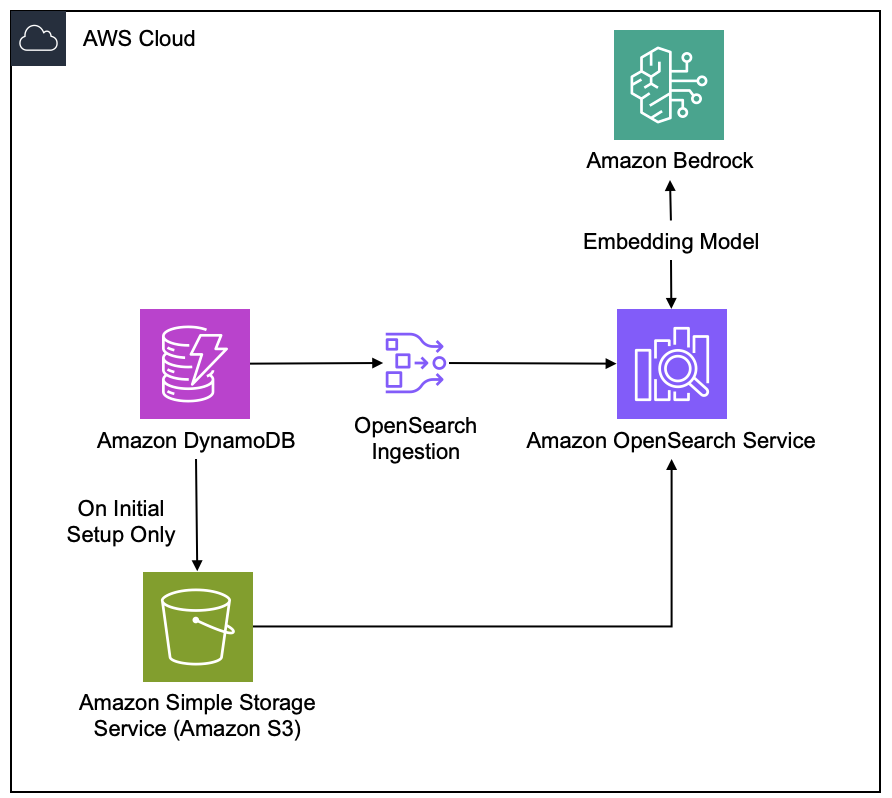
Setup: 10M vectors; 768 dimensions; K: 10 (retrieve top K values); No QuantizationResults Recall: ~90% Throughput: 12,763 QPS P99 Latency: 7.8 ms Cost: $1,643 / Month for 1Y full up front Estimating the AWS cost for this case is not trivial. The write-path includes DynamoDB (storage+ops), DynamoDB streams, S3 (storage, API), OpenSearch (data nodes, master nodes, EBS), and the OSIS pipeline. To read more on the pricing of Amazon Zero ETL, see Implementing search on Amazon DynamoDB data using zero-ETL integration with Amazon OpenSearch service. Code Examples Note: The exact JSON format might change in the next few months. 1. Enabling a Vector Index You can enable vector indexing during
CreateTable or via
UpdateTable. Note the new
VectorSecondaryIndexUpdates parameter. // Adding
a vector index to an existing table { "TableName":
"ProductCatalog", "AttributeDefinitions": [ {"AttributeName":
"ProductEmbedding", "AttributeType": "V"} ],
"VectorSecondaryIndexUpdates": [ { "Create": { "IndexName":
"VectorIdx", "VectorAttribute": { "AttributeName":
"ProductEmbedding", "Dimensions": 768 }, "IndexOptions": {
"SimilarityFunction": "COSINE", "M": 32, "ef_construction": 256 } }
} ] } Pro Tip: You will get the best
results with ScyllaDB’s optimized “V” (Vector)
type. Although you can use standard DynamoDB Lists, the
“V” type will store data as a tight array of 32-bit floats – and
that saves storage while boosting performance. 2. Performing a
Vector Search To search, use the Query operation with the ScyllaDB
VectorSearch parameter. { "TableName":
"ProductCatalog", "IndexName": "VectorIdx", "VectorSearch": {
"QueryVector": [0.12, 0.05, ..., 0.88], "Oversampling": 1.5 },
"Limit": 10, "ReturnVectorSearchSimilarity": "SIMILARITY" }
Example Use Cases Semantic Product Search Instead of relying on
exact keyword matches, users can find products based on intent. For
example, a search for “waterproof rugged hiking gear” can surface
relevant items even if those exact words aren’t in the title. RAG
(Retrieval-Augmented Generation) For knowledge bases, precision is
non-negotiable. Using the High Recall
configuration, ScyllaDB delivers 99.2% recall. That way, the LLM
receives the most accurate context possible for generating
responses. Semantic Deduplication At the Max
Throughput end of the spectrum, ScyllaDB can quickly scan
millions of incoming vectors to find near-duplicates. That prevents
redundant data from cluttering your system – reducing costs and
improving performance. Conclusion With ScyllaDB, DynamoDB users now
have a “fast track” to AI-ready infrastructure. By unifying storage
and vector search into a single API, you eliminate the operational
tax of “Zero ETL” without sacrificing the sub-millisecond
performance ScyllaDB is known for. ScyllaDB Vector Search Benchmark: 10M Vectors on a Compact Cluster
Even a small, compact setup achieved up to 12,840 QPS at k=10 with a serial P99 latency of 5.5 ms Our 1-billion-vector benchmark demonstrated that ScyllaDB Vector Search can sustain 252,000 QPS with 2 ms P99 latency across a large-scale deployment. But not every workload starts at a billion vectors. Many production use cases (e.g., product catalogs, knowledge bases for RAG, and semantic caches) live comfortably in the 10–100 million range. This post presents a smaller benchmark: a 10-million-vector dataset of 768-dimensional Cohere embeddings on a compact five-node cluster. It used three modest storage nodes and two memory-optimized search nodes, all running on AWS Graviton. We explore four index configurations that span the recall-throughput spectrum, from near-perfect recall to maximum throughput. The results show that even this small setup can deliver up to 12,840 QPS at k=10 with a serial P99 latency of 5.5 ms — without any quantization. Architecture at a Glance First, some background. ScyllaDB Vector Search separates storage and indexing responsibilities while keeping the system unified from the user’s perspective. The ScyllaDB storage nodes hold both the structured attributes and the vector embeddings in the same distributed table. Meanwhile, a dedicated Vector Store service — implemented in Rust and powered by the USearch engine — consumes updates from ScyllaDB via CDC and builds approximate nearest neighbor (ANN) indexes in memory. Queries are issued through standard CQL: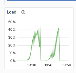
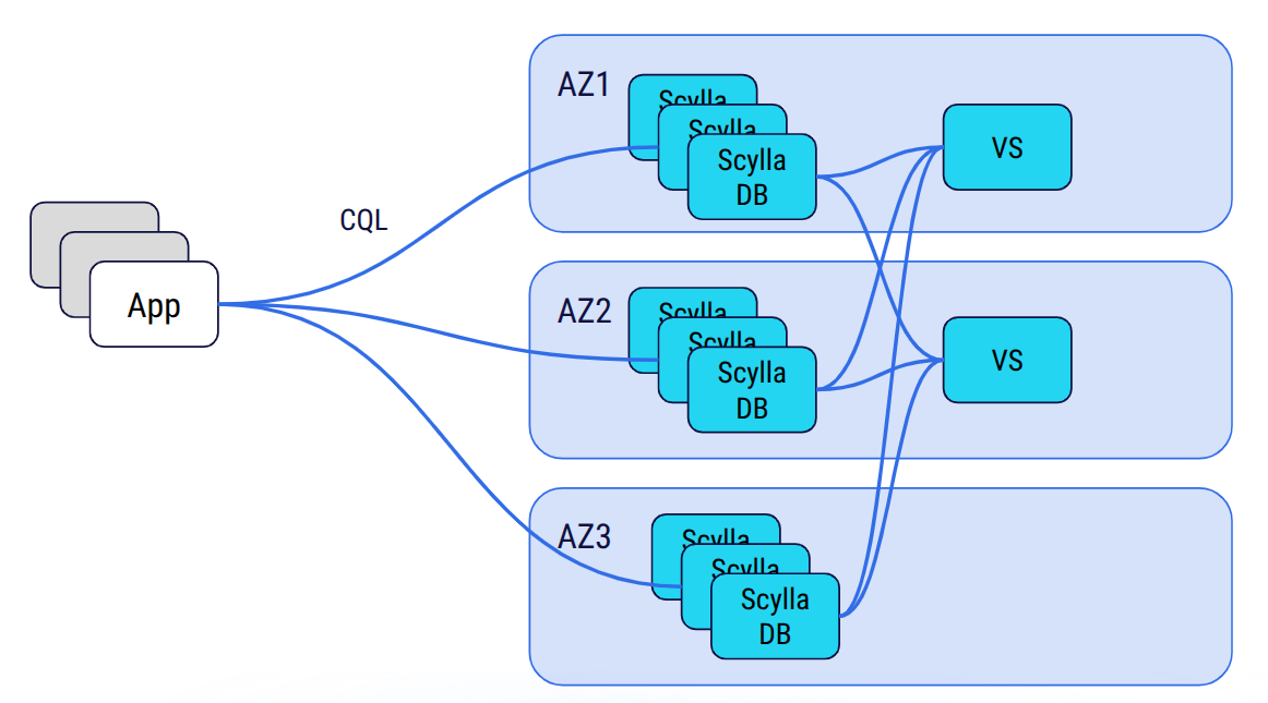
SELECT … ORDER BY vector_column ANN OF
? LIMIT k;
The queries are internally routed to the Vector
Store service, which performs the HNSW similarity search and
returns the candidate rows. This design allows each layer to scale
independently, optimizing for its own workload characteristics and
eliminating resource interference. For a detailed architectural
deep-dive, see the
1-billion-vector benchmark and the technical blog
Building a Low-Latency Vector Search Engine for ScyllaDB.
Benchmark Setup Here’s a look at the dataset and hardware used for
the benchmark. Dataset Property
Value Vectors 10,000,000
Dimensions 768 Embedding model
Cohere Similarity function COSINE
Quantization None (f32) Hardware
Role Instance
vCPUs RAM Count
Storage nodes i8g.large 2 16 GB 3 Search
nodes r7g.2xlarge 8 64 GB 2 With 768-dimensional f32
vectors and M values up to 64, the in-memory index size can be
estimated as: Memory ≈ N × (D × 4 + M × 16) × 1.2 For the largest
configuration (M=64): 10M × (768 × 4 + 64 × 16) × 1.2 ≈ 49
GB, which fits comfortably in the 64 GB of a single
r7g.2xlarge search node. No quantization is needed at this
scale. Experiments We tested four HNSW index
configurations, progressively lowering graph connectivity (M) and
search effort (ef_search) to shift the balance from
recall toward throughput. Experiment
M ef_construction
ef_search k tested
#1 (high quality) 64 384 192 100, 10
#2 (balanced) 32 256 128 100, 10
#3 (high throughput) 24 256 64 100, 10
#4 (max throughput) 20 256 48 10 The three HNSW
parameters control different aspects of the index:
M
(maximum_node_connections): Maximum edges per node in
the HNSW graph. Higher values create a richer, better-connected
graph that improves recall at the cost of more memory and slower
inserts and queries. ef_construction
(construction_beam_width): Controls how thoroughly the
algorithm searches for the best neighbors when inserting a new
vector. Higher values produce a higher-quality graph but slow down
index building. This is a one-time cost.
ef_search
(search_beam_width): The main tuning knob for query
performance. Controls the size of the candidate beam during search.
Higher values evaluate more candidates, which improves recall but
increases query latency. Since vector index options cannot be
changed after creation, each experiment required dropping and
recreating the index. Here are the CQL statements used: --
Experiment #1: M=64, ef_construction=384, ef_search=192 CREATE
CUSTOM INDEX vdb_bench_collection_vector_idx ON
vdb_bench.vdb_bench_collection (vector) USING 'vector_index' WITH
OPTIONS = { 'search_beam_width': '192', 'construction_beam_width':
'384', 'maximum_node_connections': '64', 'similarity_function':
'COSINE' }; -- Experiment #2: M=32, ef_construction=256,
ef_search=128 CREATE CUSTOM INDEX vdb_bench_collection_vector_idx
ON vdb_bench.vdb_bench_collection (vector) USING 'vector_index'
WITH OPTIONS = { 'search_beam_width': '128',
'construction_beam_width': '256', 'maximum_node_connections': '32',
'similarity_function': 'COSINE' }; -- Experiment #3: M=24,
ef_construction=256, ef_search=64 CREATE CUSTOM INDEX
vdb_bench_collection_vector_idx ON vdb_bench.vdb_bench_collection
(vector) USING 'vector_index' WITH OPTIONS = { 'search_beam_width':
'64', 'construction_beam_width': '256', 'maximum_node_connections':
'24', 'similarity_function': 'COSINE' }; -- Experiment #4: M=20,
ef_construction=256, ef_search=48 CREATE CUSTOM INDEX
vdb_bench_collection_vector_idx ON vdb_bench.vdb_bench_collection
(vector) USING 'vector_index' WITH OPTIONS = { 'search_beam_width':
'48', 'construction_beam_width': '256', 'maximum_node_connections':
'20', 'similarity_function': 'COSINE' }; The benchmark was
run using VectorDBBench with
the upcoming ScyllaDB Python driver built on a Rust core (a dev
version is available at
python-rs-driver). VectorDBBench ramps concurrency from 1 to
150 concurrent search clients and measures QPS, P99 and average
latency at each level. A separate serial run of 1,000 queries
measures recall and nDCG against brute-force ground truth. Results
Peak QPS Comparison To start our analysis, let’s examine the
maximum throughput that each index configuration can sustain under
peak concurrency. When strictly looking at the highest throughput
achieved:
The bar chart highlights the dramatic impact of index parameters at
k=10: throughput rises sharply as the index becomes lighter. At
k=100, the differences are much smaller; all configurations cluster
between 2,300 and 3,000 QPS. QPS vs Concurrency The chart below
shows how each index configuration scales as concurrency ramps from
1 to 150 clients.
At k=10, the lighter configurations (Experiments
#3 and #4) scale nearly linearly up to 60–80 concurrent clients
before saturating. Experiment #4 demonstrates the benefit of a
leaner graph: it achieves 5.5X higher peak QPS
than Experiment #1 at k=10. At k=100, all
configurations converge to a narrower throughput band (2,300–3,025
QPS). This shows that retrieving 100 neighbors dominates the
per-query cost regardless of index parameters. P99 and Average
Latency vs Concurrency As expected, increasing throughput adds
queuing delay, and that leads to higher tail latencies.
<!-- Note: The original document had 6 images. The source note
lists the order as 4-1-2-3-5-6. The text contains 7 [image]
placeholders. Based on the document's structure, I will assume the
sixth placeholder corresponds to the last chart (Average Latency)
and omit the extra placeholder, as the source note only accounts
for six images. I will adjust the numbering below. The original
list was 4-1-2-3-5-6. I will use the final placeholder (Image 6
from source) here. The next section has another chart, so I will
add a seventh placeholder and mark it as 'Source Unknown'.
Lighter configurations start at dramatically lower baseline
latencies. Experiment #4 maintains sub-6 ms P99 latency up to 30
concurrent clients, while Experiment #1 starts above 13 ms, even at
concurrency 1. All configurations show latency rising
proportionally once throughput saturates. This is the expected
queuing behavior when the system is at capacity. QPS vs P99 Latency
(Pareto View) Plotting throughput directly against tail latency
provides a Pareto frontier of our benchmark configurations:
This view makes the operational trade-off easier to read than the
concurrency charts alone. At k=10, Experiments #3 and #4 push the
frontier outward, with much higher QPS at the same or lower tail
latency. At k=100, the frontier is tighter, which again shows that
returning more neighbors dominates the total cost per query. Recall
vs Peak QPS Finally, plotting recall helps select the optimal index
strategy based on business requirements:
This chart summarizes the core choice in a single picture: should
you spend compute on accuracy or throughput? Experiment #1 sits at
the high-recall end, Experiment #4 at the high-throughput end, and
Experiment #2 emerges as the practical middle ground for workloads
that need both. Scenario Analysis With the charts above as a visual
reference, let’s examine the three main usage scenarios that emerge
from the data. Scenario 1: Maximum Throughput Experiments #3 (M=24,
ef_search=64) and #4 (M=20, ef_search=48) target workloads where
throughput is the primary objective and moderate recall is
acceptable — for example, coarse candidate retrieval stages in
recommendation pipelines or semantic deduplication. At
k=10, Experiment #4 reached a peak of
12,840 QPS at concurrency 100, with a serial P99
latency of just 5.5 ms and recall of
92.0%. Experiment #3 achieved 9,719
QPS with marginally better recall at
95.0% and a serial P99 of 6.0 ms.
Even at k=100, these lightweight configurations
delivered competitive throughput: Experiment #3 peaked at
3,025 QPS (87.9% recall), which is comparable to
the heavier configurations. Retrieval of 100 neighbors per query
inherently requires more work, which limits the throughput range
across all configurations. Scenario 2: High Recall Experiment #1
(M=64, ef_search=192) prioritizes accuracy for applications that
cannot tolerate missed results (e.g., high-fidelity semantic
search, retrieval-augmented generation [RAG] pipelines, or
compliance-sensitive retrieval). At k=10, the
system delivered 99.2% recall and 99.1%
nDCG — essentially indistinguishable from exact
brute-force search. Peak QPS reached 2,324 with a
serial P99 latency of 14.6 ms. At
k=100, recall was 96.8% with
2,345 QPS and a serial P99 of 15.2
ms. The higher latency and lower throughput are a direct
consequence of the richer graph (64 connections per node) and wider
search beam (192 candidates), which evaluate substantially more
distance computations per query. Scenario 3: Balanced Experiment #2
(M=32, ef_search=128) takes the middle ground, offering strong
recall with significantly better throughput than the high-recall
configuration. At k=10, it achieved 97.7%
recall with 4,897 QPS — roughly double
the throughput of Experiment #1, with only a 1.5 percentage-point
recall reduction. The serial P99 was 8.7 ms. At
k=100, recall was 92.0% with
2,975 QPS and a serial P99 of 9.6
ms. This configuration represents a practical sweet spot
for many production deployments where both recall and throughput
matter. Summary Tables k=100 Metric #1
M=64 ef_s=192 #2 M=32 ef_s=128 #3
M=24 ef_s=64 Peak QPS 2,345 (c=150) 2,975
(c=40) 3,025 (c=40) QPS @ c=10 947 1,314 1,489
Serial P99 Latency 15.2 ms 9.6 ms 7.8 ms
P99 Latency @ c=1 15.5 ms 9.9 ms 8.1 ms
P99 Latency @ c=100 81.2 ms 49.9 ms 49.6 ms
Recall 96.8% 92.0% 87.9% nDCG
97.3% 93.1% 89.7% k=10 Metric #1 M=64
ef_s=192 #2 M=32 ef_s=128 #3 M=24
ef_s=64 #4 M=20 ef_s=48 Peak
QPS 2,324 (c=100) 4,897 (c=80) 9,719 (c=80) 12,840 (c=100)
QPS @ c=10 1,054 1,602 2,046 2,311 Serial
P99 Latency 14.6 ms 8.7 ms 6.0 ms 5.5 ms P99
Latency @ c=1 14.0 ms 8.5 ms 6.2 ms 5.5 ms P99
Latency @ c=100 81.0 ms 38.1 ms 18.0 ms 12.3 ms
Recall 99.2% 97.7% 95.0% 92.0%
nDCG 99.1% 97.6% 94.9% 92.0% Key Takeaways
k=10 vs k=100: At k=10, lighter index parameters
yield massive throughput gains (up to 5.5X) with modest recall
loss. At k=100, all configurations converge to a narrow QPS band
(~1.3X range) because retrieving more neighbors dominates per-query
cost. Recall trade-offs are favorable: At k=10,
recall drops only 7.2 pp (99.2% to 92.0%) for a 5.5X QPS increase.
At k=100, the trade-off is steeper: 8.9 pp for just 1.3X gain.
Latency tracks index weight: Serial P99 drops from
14.6 ms to 5.5 ms at k=10, and from 15.2 ms to 7.8 ms at k=100, as
lighter graphs require fewer distance computations.
Saturation points differ: Experiments #1–#3
plateau around c=40–80; Experiment #4 scales further to c=100
before saturating, reflecting its lower per-query compute cost.
Conclusion These results show that ScyllaDB Vector Search delivers
strong performance even on a compact, five-node cluster with 10
million 768-dimensional vectors. A pair of r7g.2xlarge search nodes
provides enough memory to hold the full HNSW index at f32 precision
– without requiring any quantization. The three storage nodes with
replication factor 3, combined with vector search nodes distributed
across availability zones, also provide high availability. The
system is designed to tolerate node failures without data loss or
service interruption. Depending on the index configuration, the
system can prioritize near-perfect recall (99.2% at k=10) or
maximize throughput (12,840 QPS at k=10 with 92% recall), with
practical balanced options in between. This 10M scenario represents
the accessible end of the scale. For workloads that push into
hundreds of millions or billions of vectors, quantization,
additional search nodes and larger instances extend the same
architecture. See the ScyllaDB
1-billion-vector benchmark for results at extreme scale, and
look for our upcoming 100-million-vector benchmark
post. At K=10, the performance bottleneck resides within the vector
index nodes, leaving ScyllaDB with significant headroom. This means
you can likely add a Vector Search index to your cluster and
continue running a similar workload on your existing ScyllaDB
infrastructure – without needing to scale your database
nodes. The full Jupyter notebook with interactive charts and all
data is available
in this repository. Ready to try it yourself? Follow the
ScyllaDB Vector Search Quick Start Guide to get started. 
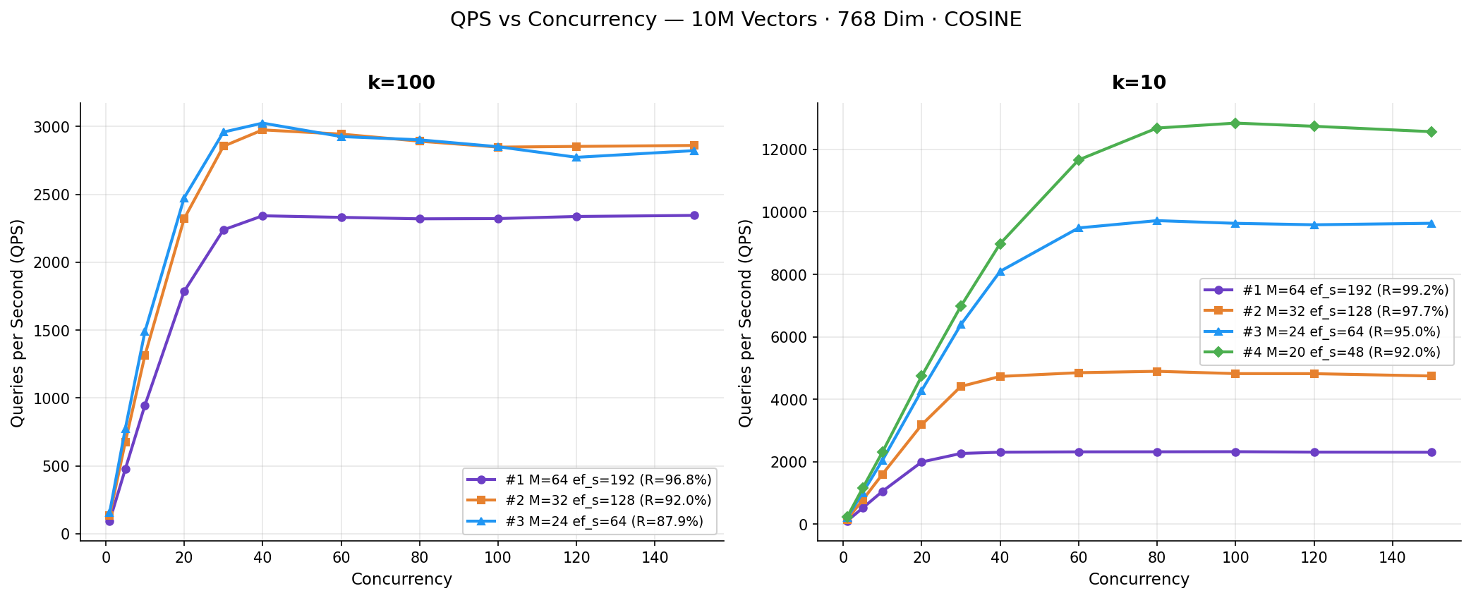
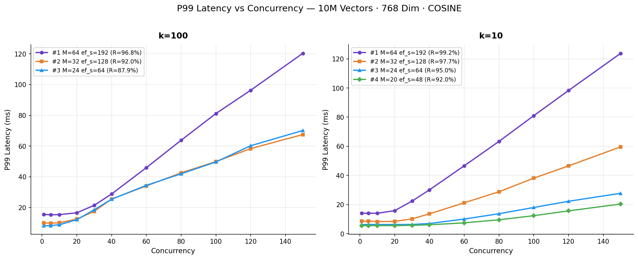
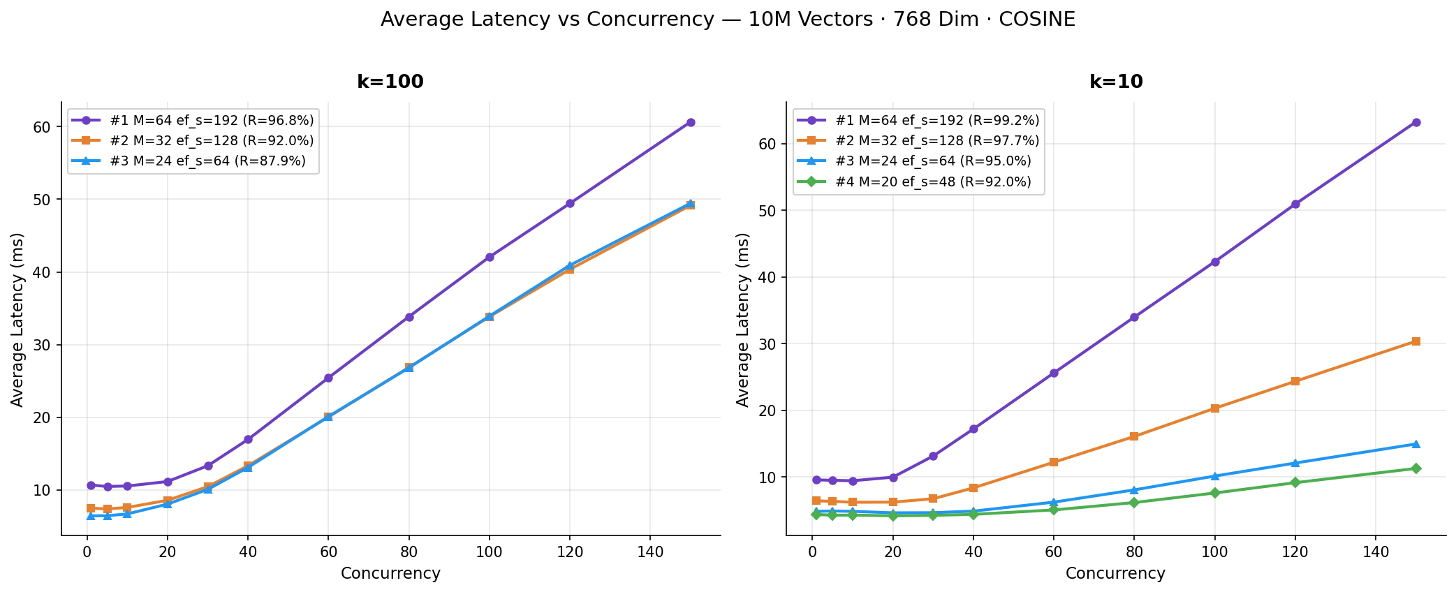
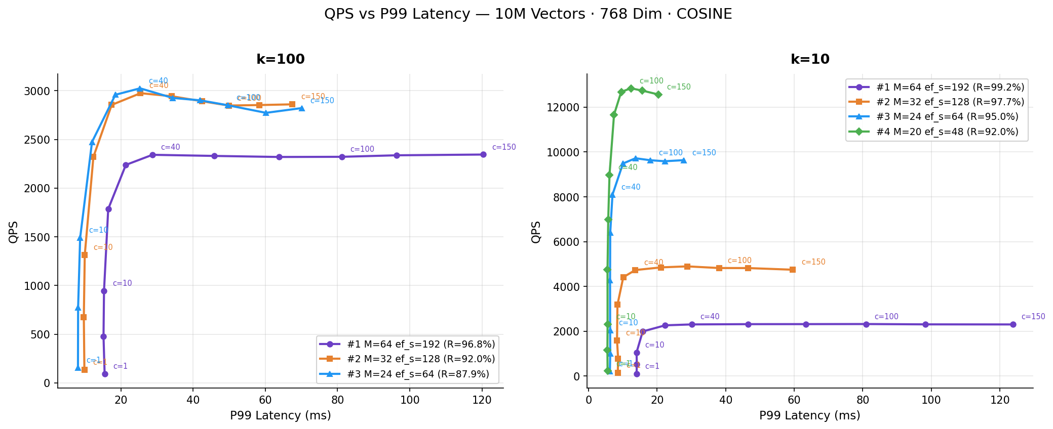
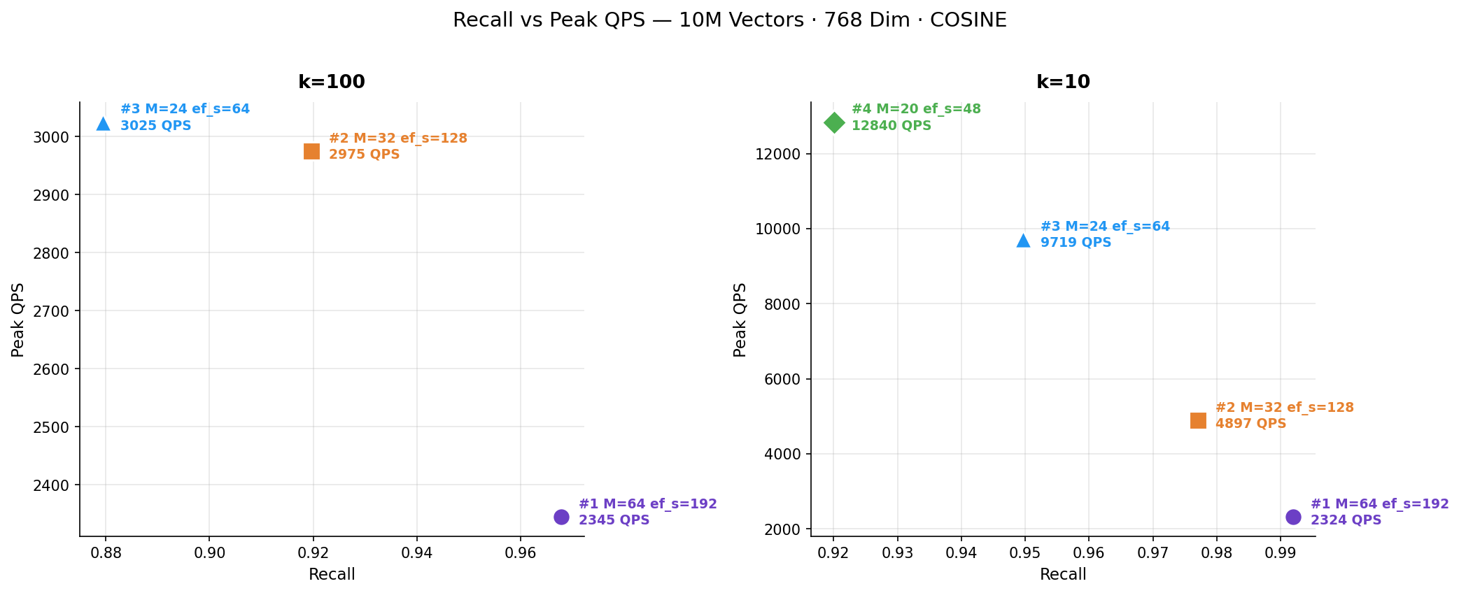