Freezing streaming data into Apache Iceberg™—Part 1: Using Apache Kafka®Connect Iceberg Sink Connector

16 December 2025, 1:00 pm by Apache Cassandra - Instaclustr

Ever since the first distributed system—i.e. 2 or more computers networked together (in 1969)—there has been the problem of distributed data consistency: How can you ensure that data from one computer is available and consistent with the second (and more) computers? This problem can be uni-directional (one computer is considered the source of truth, others are just copies), or bi-directional (data must be synchronized in both directions across multiple computers). 

Some approaches to this problem I’ve come across in the last 8 years include Kafka Connect (for elegantly solving the heterogeneous many-to-many integration problem by streaming data from source systems to Kafka and from Kafka to sink systems, some earlier blogs on Apache Camel Kafka Connectors and a blog series on zero-code data pipelines), MirrorMaker2 (MM2, for replicating Kafka clusters, a 2 part blog series), and Debezium (Change Data Capture/CDC, for capturing changes from databases as streams and making them available in downstream systems, e.g. for Apache Cassandra and PostgreSQL)—MM2 and Debezium are actually both built on Kafka Connect.  

Recently, some “sink” systems have been taking over responsibility for streaming data from Kafka into themselves, e.g. OpenSearch pull-based ingestion (c.f. OpenSearch Sink Connector), and the ClickHouse Kafka Table Engine (c.f. ClickHouse Sink Connector). These “pull-based” approaches are potentially easier to configure and don’t require running a separate Kafka Connect cluster and sink connectors, but some downsides may be that they are not as reliable or independently scalable, and you will need to carefully monitor and scale them to ensure they perform adequately.  

And then there’s “zero-copy” approaches—these rely on the well-known computer science trick of sharing a single copy of data using references (or pointers), rather than duplicating the data. This idea has been around for almost as long as computers, and is still widely applicable, as we’ll see in part 2 of the blog. 

The distributed data use case we’re going to explore in this 2-part blog series is streaming Apache Kafka data into Apache Iceberg, or “Freezing streaming Apache Kafka data into an (Apache) Iceberg”! In part 1 we’ll introduce Apache Iceberg and look at the first approach for “freezing” streaming data using the Kafka Connect Iceberg Sink Connector. 

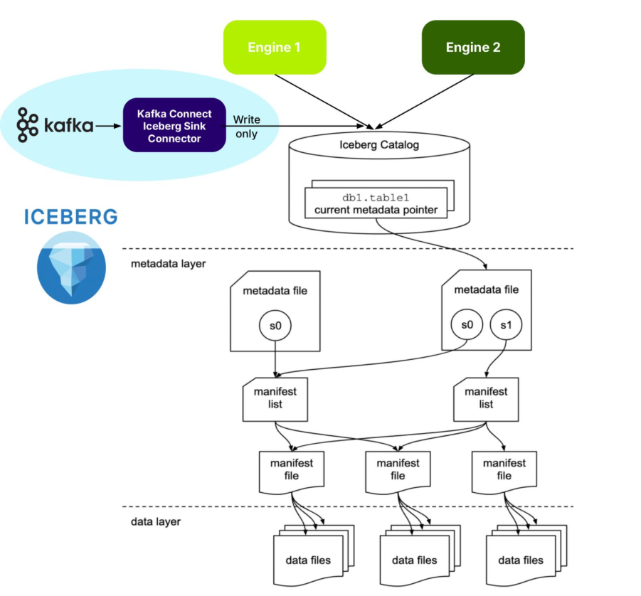
Apache Iceberg is an open source specification open table format optimized for column-oriented workloads, supporting huge analytic datasets. It supports multiple different concurrent engines that can insert and query table data using SQL—and Iceberg is organized like, well, an iceberg! 

The tip of the Iceberg is the Catalog. An Iceberg Catalog acts as a central metadata repository, tracking the current state of Iceberg tables, including their names, schemas, and metadata file locations. It serves as the “single source of truth” for a data Lakehouse, enabling query engines to find the correct metadata file for a table to ensure consistent and atomic read/write operations.  

Just under the water, the next layer is the metadata layer. The Iceberg metadata layer tracks the structure and content of data tables in a data lake, enabling features like efficient query planning, versioning, and schema evolution. It does this by maintaining a layered structure of metadata files, manifest lists, and manifest files that store information about table schemas, partitions, and data files, allowing query engines to prune unnecessary files and perform operations atomically. 

The data layer is at the bottom. The Iceberg data layer is the storage component where the actual data files are stored. It supports different storage backends, including cloud-based object storage like Amazon S3 or Google Cloud Storage, or HDFS. It uses file formats like Parquet or Avro. Its main purpose is to work in conjunction with Iceberg’s metadata layer to manage table snapshots and provide a more reliable and performant table format for data lakes, bringing data warehouse features to large datasets. 

As shown in the above diagram, Iceberg supports multiple different engines, including Apache Spark and ClickHouse. Engines provide the “database” features you would expect, including:  

• Data Management 

• ACID Transactions 

• Query Planning and Optimization 

• Schema Evolution 

• And more! 

I’ve recently been reading an excellent book on Apache Iceberg (“Apache Iceberg: The Definitive Guide”), which explains the philosophy, architecture and design, including operation, of Iceberg. For example, it says that it’s best practice to treat data lake storage as immutable—data should only be added to a Data Lake, not deleted.  So, in theory at least, writing infinite, immutable Kafka streams to Iceberg should be straightforward!  

But because it’s a complex distributed system (which looks like a database from above water but is really a bunch of files below water!), there is some operational complexity. For example, it handles change and consistency by creating new snapshots for every modification, enabling time travel, isolating readers from writes, and supporting optimistic concurrency control for multiple writers. But you need to manage snapshots (e.g. expiring old snapshots). And chapter 4 (performance optimisation) explains that you may need to worry about compaction (reducing too many small files), partitioning approaches (which can impact read performance), and handling row-level updates. The first two issues may be relevant for Kafka, but probably not the last one.  So, it looks like it’s good fit for the streaming Kafka use cases, but we may need to watch out for Iceberg management issues.  

But Apache Iceberg is “frozen”—what’s the connection to fast-moving streaming data? You certainly don’t want to collide with an iceberg from your speedy streaming “ship”—but you may want to freeze your streaming data for long-term analytical queries in the future. How can you do that without sinking? Actually, a “sink” is the first answer: A Kafka Connect Iceberg Sink Connector is the most common way of “freezing” your streaming data in Iceberg!  

Kafka Connect is the standard framework provided by Apache Kafka to move data from multiple heterogeneous source systems to multiple heterogeneous sink systems, using:  

• A Kafka cluster 

• A Kafka Connect cluster (running connectors) 

• Kafka Connect source connectors 

• Kafka topics and 

• Kafka Connect Sink Connectors 

That is, a highly decoupled approach. It provides real-time data movement with high scalability, reliability, error handling and simple transformations.   

Here’s the Kafka Connect Iceberg Sink Connector official documentation. 

It appears to be reasonably complicated to configure this sink connector; you will need to know something about Iceberg. For example, what is a “control topic”? It’s apparently used to coordinate commits for exactly-once semantics (EOS).  

The connector supports fan-out (writing to multiple Iceberg tables from one topic), fan-in (writing to one Iceberg table from multiple topics), static and dynamic routing, and filtering.  

In common with many technologies that you may want to use as Kafka Connect sinks, they may not all have good support for Kafka metadata. The KafkaMetadata Transform (which injects topic, partition, offset and timestamp properties) is only experimental at present.  

How are Iceberg tables created with the correct metadata? If you have JSON record values, then schemas are inferred by default (but may not be correct or optimal). Alternatively, explicit schemas can be included in-line or referenced from a Kafka Schema Registry (e.g. Karapace), and, as an added bonus, schema evolution is supported.  Also note that Iceberg tables may have to be manually created prior to use if your Catalog doesn’t support table auto-creation.  

From what I understood about Iceberg, to use it (e.g. for writes), you need support from an engine (e.g. to add raw data to the Iceberg warehouse, create the metadata files, and update the catalog).  How does this work for Kafka Connect? From this blog I discovered that the Kafka Connect Iceberg Sink connector is functioning as an Iceberg engine for writes, so there really is an engine, but it’s built into the connector.  

As is the case with all Kafka Connect Sink Connectors, records are available immediately they are written to Kafka topics by Kafka producers and Kafka Connect Source Connectors, i.e. records in active segments can be copied immediately to sink systems. But is the Iceberg Sink Connector real-time? Not really! The default time to write to Iceberg is every 5 minutes (iceberg.control.commit.interval-ms) to prevent multiplication of small files—something that Iceberg(s) doesn’t/don’t like (“melting”?). In practice, it’s because every data file must be tracked in the metadata layer, which impacts performance in many ways—proliferation of small files is typically addressed by optimization and compaction (e.g. Apache Spark supports Iceberg management, including these operations). 

So, unlike most Kafka Connect sink connectors, which write as quickly as possible, there will be lag before records appear in Iceberg tables (“time to freeze” perhaps)!  

The systems are separate (Kafka and Iceberg are independent), records are copied to Iceberg, and that’s it! This is a clean separation of concerns and ownership. Kafka owns the source data (with Kafka controlling data lifecycles, including record expiry), Kafka Connect Iceberg Sink Connector performs the reading from Kafka and writing to Iceberg, and is independently scalable to Kafka. Kafka doesn’t handle any of the Iceberg management.  Once the data has landed in Iceberg, Kafka has no further visibility or interest in it. And the pipeline is purely one way, write only – reads or deletes are not supported.  

Here’s a summary of this approach to freezing streams:  

1. Kafka Connect Iceberg Sink Connector shares all the benefits of the Kafka Connect framework, including scalability, reliability, error handling, routing, and transformations.  
2. At least, JSON values are required, ideally full schemas and referenced in Karapace—but not all schemas are guaranteed to work. 
3. Kafka Connect doesn’t “manage” Iceberg (e.g. automatically aggregate small files, remove snapshots, etc.) 
4. You may have to tune the commit interval – 5 minutes is the default. 
5. But it does have a built-in engine that supports writing to Iceberg. 
6. You may need to use an external tool (e.g. Apache Spark) for Iceberg management procedures. 
7. It’s write-only to Iceberg. Reads or deletes are not supported 

But what’s the best thing about the Kafka Connect Iceberg Sink Connector? It’s available now (as part of the Apache Iceberg build) and works on the NetApp Instaclustr Kafka Connect platform as a “bring your own connector”  (instructions here).  

In part 2, we’ll look at Kafka Tiered Storage and Iceberg Topics! 

The post Freezing streaming data into Apache Iceberg™—Part 1: Using Apache Kafka®Connect Iceberg Sink Connector appeared first on Instaclustr.

Netflix Live Origin

15 December 2025, 5:38 pm by Netflix TechBlog - Medium

Xiaomei Liu, Joseph Lynch, Chris Newton

Introduction

Behind the Streams: Building a Reliable Cloud Live Streaming Pipeline for Netflix introduced the architecture of the streaming pipeline. This blog post looks at the custom Origin Server we built for Live — the Netflix Live Origin. It sits at the demarcation point between the cloud live streaming pipelines on its upstream side and the distribution system, Open Connect, Netflix’s in-house Content Delivery Network (CDN), on its downstream side, and acts as a broker managing what content makes it out to Open Connect and ultimately to the client devices.

Netflix Live Origin is a multi-tenant microservice operating on EC2 instances within the AWS cloud. We lean on standard HTTP protocol features to communicate with the Live Origin. The Packager pushes segments to it using PUT requests, which place a file into storage at the particular location named in the URL. The storage location corresponds to the URL that is used when the Open Connect side issues the corresponding GET request.

Live Origin architecture is influenced by key technical decisions of the live streaming architecture. First, resilience is achieved through redundant regional live streaming pipelines, with failover orchestrated at the server-side to reduce client complexity. The implementation of epoch locking at the cloud encoder enables the origin to select a segment from either encoding pipeline. Second, Netflix adopted a manifest design with segment templates and constant segment duration to avoid frequent manifest refresh. The constant duration templates enable Origin to predict the segment publishing schedule.

Multi-pipeline and multi-region aware origin

Live streams inevitably contain defects due to the non-deterministic nature of live contribution feeds and strict real-time segment publishing timelines. Common defects include:

• Short segments: Missing video frames and audio samples.
• Missing segments: Entire segments are absent.
• Segment timing discontinuity: Issues with the Track Fragment Decode Time.

Communicating segment discontinuity from the server to the client via a segment template-based manifest is impractical, and these defective segments can disrupt client streaming.

The redundant cloud streaming pipelines operate independently, encompassing distinct cloud regions, contribution feeds, encoder, and packager deployments. This independence substantially mitigates the probability of simultaneous defective segments across the dual pipelines. Owing to its strategic placement within the distribution path, the live origin naturally emerges as a component capable of intelligent candidate selection.

The Netflix Live Origin features multi-pipeline and multi-region awareness. When a segment is requested, the live origin checks candidates from each pipeline in a deterministic order, selecting the first valid one. Segment defects are detected via lightweight media inspection at the packager. This defect information is provided as metadata when the segment is published to the live origin. In the rare case of concurrent defects at the dual pipeline, the segment defects can be communicated downstream for intelligent client-side error concealment.

Open Connect streaming optimization

When the Live project started, Open Connect had become highly optimised for VOD content delivery — nginx had been chosen many years ago as the Web Server since it is highly capable in this role, and a number of enhancements had been added to it and to the underlying operating system (BSD). Unlike traditional CDNs, Open Connect is more of a distributed origin server — VOD assets are pre-positioned onto carefully selected server machines (OCAs, or Open Connect Appliances) rather than being filled on demand.

Alongside the VOD delivery, an on-demand fill system has been used for non-VOD assets — this includes artwork and the downloadable portions of the clients, etc. These are also served out of the same nginx workers, albeit under a distinct server block, using a distinct set of hostnames.

Live didn’t fit neatly into this ‘small object delivery’ model, so we extended the proxy-caching functionality of nginx to address Live-specific needs. We will touch on some of these here related to optimized interactions with the Origin Server. Look for a future blog post that will go into more details on the Open Connect side.

The segment templates provided to clients are also provided to the OCAs as part of the Live Event Configuration data. Using the Availability Start Time and Initial Segment number, the OCA is able to determine the legitimate range of segments for each event at any point in time — requests for objects outside this range can be rejected, preventing unnecessary requests going up through the fill hierarchy to the origin. If a request makes it through to the origin, and the segment isn’t available yet, the origin server will return a 404 Status Code (indicating File Not Found) with the expiration policy of that error so that it can be cached within Open Connect until just before that segment is expected to be published.

If the Live Origin knows when segments are being pushed to it, and knows what the live edge is — when a request is received for the immediately next object, rather than handing back another 404 error (which would go all the way back through Open Connect to the client), the Live Origin can ‘hold open’ the request, and service it once the segment has been published to it. By doing this, the degree of chatter within the network handling requests that arrive early has been significantly reduced. As part of this, millisecond grain caching was added to nginx to enhance the standard HTTP Cache Control, which only works at second granularity, a long time when segments are generated every 2 seconds.

Streaming metadata enhancement

The HTTP standard allows for the addition of request and response headers that can be used to provide additional information as files move between clients and servers. The HTTP headers provide notifications of events within the stream in a highly scalable way that is independently conveyed to client devices, regardless of their playback position within the stream.

These notifications are provided to the origin by the live streaming pipeline and are inserted by the origin in the form of headers, appearing on the segments generated at that point in time (and persist to future segments — they are cumulative). Whenever a segment is received at an OCA, this notification information is extracted from the response headers and used to update an in-memory data structure, keyed by event ID; and whenever a segment is served from the OCA, the latest such notification data is attached to the response. This means that, given any flow of segments into an OCA, it will always have the most recent notification data, even if all clients requesting it are behind the live edge. In fact, the notification information can be conveyed on any response, not just those supplying new segments.

Cache invalidation and origin mask

An invalidation system has been available since the early days of the project. It can be used to “flush” all content associated with an event by altering the key used when looking up objects in cache — this is done by incorporating a version number into the cache key that can then be bumped on demand. This is used during pre-event testing so that the network can be returned to a pristine state for the test with minimal fuss.

Each segment published by the Live Origin conveys the encoding pipeline it was generated by, as well as the region it was requested from. Any issues that are found after segments make their way into the network can be remedied by an enhanced invalidation system that takes such variants into account. It is possible to invalidate (that is, cause to be considered expired) segments in a range of segment numbers, but only if they were sourced from encoder A, or from Encoder A, but only if retrieved from region X.

In combination with Open Connect’s enhanced cache invalidation, the Netflix Live Origin allows selective encoding pipeline masking to exclude a range of segments from a particular pipeline when serving segments to Open Connect. The enhanced cache invalidation and origin masking enable live streaming operations to hide known problematic segments (e.g., segments causing client playback errors) from streaming clients once the bad segments are detected, protecting millions of streaming clients during the DVR playback window.

Origin storage architecture

Our original storage architecture for the Live Origin was simple: just use AWS S3 like we do for SVOD. This served us well initially for our low-traffic events, but as we scaled up we discovered that Live streaming has unique latency and workload requirements that differ significantly from on-demand where we have significant time ahead-of-time to pre-position content. While S3 met its stated uptime guarantees, our strict 2-second retry budget inherent to Live events (where every write is critical) led us to explore optimizations specifically tailored for real-time delivery at scale. AWS S3 is an amazing object store, but our Live streaming requirements were closer to those of a global low-latency highly-available database. So, we went back to the drawing board and started from the requirements. The Origin required:

1. [HA Writes] Extremely high write availability, ideally as close to full write availability within a single AWS region, with low second replication delay to other regions. Any failed write operation within 500ms is considered a bug that must be triaged and prevented from re-occurring.
2. [Throughput] High write throughput, with hundreds of MiB replicating across regions
3. [Large Partitions] Efficiently support O(MiB) writes that accumulate to O(10k) keys per partition with O(GiB) total size per event.
4. [Strong Consistency] Within the same region, we needed read-your-write semantics to hit our <1s read delay requirements (must be able to read published segments)
5. [Origin Storm] During worst-case load involving Open Connect edge cases, we may need to handle O(GiB) of read throughput without affecting writes.

Fortunately, Netflix had previously invested in building a KeyValue Storage Abstraction that cleverly leveraged Apache Cassandra to provide chunked storage of MiB or even GiB values. This abstraction was initially built to support cloud saves of Game state. The Live use case would push the boundaries of this solution, however, in terms of availability for writes (#1), cumulative partition size (#3), and read throughput during Origin Storm (#5).

High Availability for Writes of Large Payloads

The KeyValue Payload Chunking and Compression Algorithm breaks O(MiB) work down so each part can be idempotently retried and hedged to maintain strict latency service level objectives, as well as spreading the data across the full cluster. When we combine this algorithm with Apache Cassandra’s local-quorum consistency model, which allows write availability even with an entire Availability Zone outage, plus a write-optimized Log-Structured Merge Tree (LSM) storage engine, we could meet the first four requirements. After iterating on the performance and availability of this solution, we were not only able to achieve the write availability required, but did so with a P99 tail latency that was similar to the status quo’s P50 average latency while also handling cross-region replication behind the scenes for the Origin. This new solution was significantly more expensive (as expected, databases backed by SSD cost more), but minimizing cost was not a key objective and low latency with high availability was:

High Availability Reads at Gbps Throughputs

Now that we solved the write reliability problem, we had to handle the Origin Storm failure case, where potentially dozens of Open Connect top-tier caches could be requesting multiple O(MiB) video segments at once. Our back-of-the-envelope calculations showed worst-case read throughput in the O(100Gbps) range, which would normally be extremely expensive for a strongly-consistent storage engine like Apache Cassandra. With careful tuning of chunk access, we were able to respond to reads at network line rate (100Gbps) from Apache Cassandra, but we observed unacceptable performance and availability degradation on concurrent writes. To resolve this issue, we introduced write-through caching of chunks using our distributed caching system EVCache, which is based on Memcached. This allows almost all reads to be served from a highly scalable cache, allowing us to easily hit 200Gbps and beyond without affecting the write path, achieving read-write separation.

Final Storage Architecture

In the final storage architecture, the Live Origin writes and reads to KeyValue, which manages a write-through cache to EVCache (memcached) and implements a safe chunking protocol that spreads large values and partitions them out across the storage cluster (Apache Cassandra). This allows almost all read load to be handled from cache, with only misses hitting the storage. This combination of cache and highly available storage has met the demanding needs of our Live Origin for over a year now.

Delivering this consistent low latency for large writes with cross-region replication and consistent write-through caching to a distributed cache required solving numerous hard problems with novel techniques, which we plan to share in detail during a future post.

Scalability and scalable architecture

Netflix’s live streaming platform must handle a high volume of diverse stream renditions for each live event. This complexity stems from supporting various video encoding formats (each with multiple encoder ladders), numerous audio options (across languages, formats, and bitrates), and different content versions (e.g., with or without advertisements). The combination of these elements, alongside concurrent event support, leads to a significant number of unique stream renditions per live event. This, in turn, necessitates a high Requests Per Second (RPS) capacity from the multi-tenant live origin service to ensure publishing-side scalability.

In addition, Netflix’s global reach presents distinct challenges to the live origin on the retrieval side. During the Tyson vs. Paul fight event in 2024, a historic peak of 65 million concurrent streams was observed. Consequently, a scalable architecture for live origin is essential for the success of large-scale live streaming.

Scaling architecture

We chose to build a highly scalable origin instead of relying on the traditional origin shields approach for better end-to-end cache consistency control and simpler system architecture. The live origin in this architecture directly connects with top-tier Open Connect nodes, which are geographically distributed across several sites. To minimize the load on the origin, only designated nodes per stream rendition at each site are permitted to directly fill from the origin.

While the origin service can autoscale horizontally using EC2 instances, there are other system resources that are not autoscalable, such as storage platform capacity and AWS to Open Connect backbone bandwidth capacity. Since in live streaming, not all requests to the live origin are of the same importance, the origin is designed to prioritize more critical requests over less critical requests when system resources are limited. The table below outlines the request categories, their identification, and protection methods.

Publishing isolation

Publishing traffic, unlike potentially surging CDN retrieval traffic, is predictable, making path isolation a highly effective solution. As shown in the scalability architecture diagram, the origin utilizes separate EC2 publishing and CDN stacks to protect the latency and failure-sensitive origin writes. In addition, the storage abstraction layer features distinct clusters for key-value (KV) read and KV write operations. Finally, the storage layer itself separates read (EVCache) and write (Cassandra) paths. This comprehensive path isolation facilitates independent cloud scaling of publishing and retrieval, and also prevents CDN-facing traffic surges from impacting the performance and reliability of origin publishing.

Priority rate limiting

Given Netflix’s scale, managing incoming requests during a traffic storm is challenging, especially considering non-autoscalable system resources. The Netflix Live Origin implemented priority-based rate limiting when the underlying system is under stress. This approach ensures that requests with greater user impact are prioritized to succeed, while requests with lower user impact are allowed to fail during times of stress in order to protect the streaming infrastructure and are permitted to retry later to succeed.

Leveraging Netflix’s microservice platform priority rate limiting feature, the origin prioritizes live edge traffic over DVR traffic during periods of high load on the storage platform. The live edge vs. DVR traffic detection is based on the predictable segment template. The template is further cached in memory on the origin node to enable priority rate limiting without access to the datastore, which is valuable especially during periods of high datastore stress.

To mitigate traffic surges, TTL cache control is used alongside priority rate limiting. When the low-priority traffic is impacted, the origin instructs Open Connect to slow down and cache identical requests for 5 seconds by setting a max-age = 5s and returns an HTTP 503 error code. This strategy effectively dampens traffic surges by preventing repeated requests to the origin within that 5-second window.

The following diagrams illustrate origin priority rate limiting with simulated traffic. The nliveorigin_mp41 traffic is the low-priority traffic and is mixed with other high-priority traffic. In the first row: the 1st diagram shows the request RPS, the 2nd diagram shows the percentage of request failure. In the second row, the 1st diagram shows datastore resource utilization, and the 2nd diagram shows the origin retrieval P99 latency. The results clearly show that only the low-priority traffic (nliveorigin_mp41) is impacted at datastore high utilization, and the origin request latency is under control.

404 storm and cache optimization

Publishing isolation and priority rate limiting successfully protect the live origin from DVR traffic storms. However, the traffic storm generated by requests for non-existent segments presents further challenges and opportunities for optimization.

The live origin structures metadata hierarchically as event > stream rendition > segment, and the segment publishing template is maintained at the stream rendition level. This hierarchical organization allows the origin to preemptively reject requests with an HTTP 404(not found)/410(Gone) error, leveraging highly cacheable event and stream rendition level metadata, avoiding unnecessary queries to the segment level metadata:

• If the event is unknown, reject the request with 404
• If the event is known, but the segment request timing does not match the expected publishing timing, reject the request with 404 and cache control TTL matching the expected publishing time
• If the event is known, the requested segment is never generated or misses the retry deadline, reject the request with a 410 error, preventing the client from repeatedly requesting

At the storage layer, metadata is stored separately from media data in the control plane datastore. Unlike the media datastore, the control plane datastore does not use a distributed cache to avoid cache inconsistency. Event and rendition level metadata benefits from a high cache hit ratio when in-memory caching is utilized at the live origin instance. During traffic storms involving non-existent segments, the cache hit ratio for control plane access easily exceeds 90%.

The use of in-memory caching for metadata effectively handles 404 storms at the live origin without causing datastore stress. This metadata caching complements the storage system’s distributed media cache, providing a complete solution for traffic surge protection.

Summary

The Netflix Live Origin, built upon an optimized storage platform, is specifically designed for live streaming. It incorporates advanced media and segment publishing scheduling awareness and leverages enhanced intelligence to improve streaming quality, optimize scalability, and improve Open Connect live streaming operations.

Acknowledgement

Many teams and stunning colleagues contributed to the Netflix live origin. Special thanks to Flavio Ribeiro for advocacy and sponsorship of the live origin project; to Raj Ummadisetty, Prudhviraj Karumanchi for the storage platform; to Rosanna Lee, Hunter Ford, and Thiago Pontes for storage lifecycle management; to Ameya Vasani for e2e test framework; Thomas Symborski for orchestrator integration; to James Schek for Open Connect integration; to Kevin Wang for platform priority rate limit; to Di Li, Nathan Hubbard for origin scalability testing.

Netflix Live Origin was originally published in Netflix TechBlog on Medium, where people are continuing the conversation by highlighting and responding to this story.

Stay ahead with Apache Cassandra®: 2025 CEP highlights

8 December 2025, 12:00 pm by Apache Cassandra - Instaclustr

Apache Cassandra® committers are working hard, building new features to help you more seamlessly ease operational challenges of a distributed database. Let’s dive into some recently approved CEPs and explain how these upcoming features will improve your workflow and efficiency.

CEP stands for Cassandra Enhancement Proposal. They are the process for outlining, discussing, and gathering endorsements for a new feature in Cassandra. They’re more than a feature request; those who put forth a CEP have intent to build the feature, and the proposal encourages a high amount of collaboration with the Cassandra contributors.

The CEPs discussed here were recently approved for implementation or have had significant progress in their implementation.  As with all open-source development, inclusion in a future release is contingent upon successful implementation, community consensus, testing, and approval by project committers.

With collaboration from NetApp Instaclustr, CEP-42, and subsequent iterations, delivers schema level constraints giving Cassandra users and operators more control over their data. Adding constraints on the schema level means that data can be validated at write time and send the appropriate error when data is invalid.

Constraints are defined in-line or as a separate definition. The inline style allows for only one constraint while a definition allows users to define multiple constraints with different expressions.

The scope of this CEP-42 initially supported a few constraints that covered the majority of cases, but in follow up efforts the expanded list of support includes scalar (>, <, >=, <=), LENGTH(), OCTET_LENGTH(), NOT NULL, JSON(), REGEX(). A user is also able to define their own constraints if they implement it and put them on Cassandra’s class path.

A simple example of an in-line constraint:

CREATE TABLE users (

username text PRIMARY KEY,

age int CHECK age >= 0 and age < 120

);

Constraints are not supported for UDTs (User-Defined Types) nor collections (except for using NOT NULL for frozen collections).

Enabling constraints closer to the data is a subtle but mighty way for operators to ensure that data goes into the database correctly. By defining rules just once, application code is simplified, more robust, and prevents validation from being bypassed. Those who have worked with MySQL, Postgres, or MongoDB will enjoy this addition to Cassandra.

The cassandra.yaml file holds important settings for storage, memory, replication, compaction, and more. It’s no surprise that the average size of the file around 1,000 lines (though, yes—most are comments). CEP-51 enables splitting the cassandra.yaml configuration into multiple files using includes semantics. From the outside, this feels like a small change, but the implications are huge if a user chooses to opt-in.

In general, the size of the configuration file makes it difficult to manage and coordinate changes. It’s often the case that multiple teams manage various aspects of the single file. In addition, cassandra.yaml permissions are readable for those with access to this file, meaning private information like credentials are comingled with all other settings. There is risk from an operational and security standpoint.

Enabling the new semantics and therefore modularity for the configuration file eases management, deployment, complexity around environment-specific settings, and security in one shot. The configuration file follows the principle of least privilege once the cassandra.yaml is broken up into smaller, well-defined files; sensitive configuration settings are separated out from general settings with fine-grained access for the individual files. With the feature enabled, different development teams are better equipped to deploy safely and independently.

If you’ve deployed your Cassandra cluster on the NetApp Instaclustr platform, the cassandra.yaml file is already configured and managed for you. We pride ourselves on making it easy for you to get up and running fast.

With extensive review by the NetApp Instaclustr team and Stefan Miklosovic, CEP-52 introduces schema annotations in CQL allowing in-line comments and labels of schema elements such as keyspaces, tables, columns, and User Defined Types (UDT). Users can easily define and alter comments and labels on these elements. They can be copied over when desired using CREATE TABLE LIKE syntax. Comments are stored as plain text while labels are stored as structured metadata.

Comments and labels serve different annotation purposes: Comments document what a schema object is for, whereas labels describe how sensitive or controlled it is meant to be. For example, labels can be used to identify columns as “PII” or “confidential”, while the comment on that column explains usage, e.g. “Last login timestamp.”

Users can query these annotations. CEP-52 defines two new read-only tables (system_views.schema_comments and system_views.schema_security_labels) to store comments and security labels so objects with comments can be returned as a list or a user/machine process can query for specific labels, beneficial for auditing and classification. Note that adding security labels are descriptive metadata and do not enforce access control to the data.

Sidecar is an auxiliary component in the Cassandra ecosystem that exposes cluster management and streaming capabilities through APIs. Introducing rolling restarts through Sidecar, this feature is designed to provide operators with more efficient and safer restarts without cluster-wide downtime. More specifically, operators can monitor, pause, resume, and abort restarts all through an API with configurable options if restarts fail.

Rolling restarts brings operators a step closer to cluster-wide operations and lifecycle management via Sidecar. Operators will be able to configure the number of nodes to restart concurrently with minimal risk as this CEP unleashes clear states as a node progresses through a restart. Accounting for a variety of edge cases, an operator can feel assured that, for example, a non-functioning sidecar won’t derail operations.

The current process for restarting a node is a multi-step, manual process, which does not scale for large cluster sizes (and is also tedious for small clusters). Restarting clusters previously lacked a streamlined approach as each node needed to be restarted one at a time, making the process time-intensive and error-prone.

Though Sidecar is still considered WIP, it’s got big plans to improve operating large clusters!

The NetApp Instaclustr Platform, in conjunction with our expert TechOps team already orchestrates these laborious tasks for our Cassandra customers with a high level of care to ensure their cluster stays online. Restarting or upgrading your Cassandra nodes is a huge pain-point for operators, but it doesn’t have to be when using our managed platform (with round-the-clock support!)

CEP-54, with NetApp Instaclustr’s collaboration, aims to add support Zstd with dictionary compression for SSTables. Zstd, or Zstandard, is a fast, lossless data compression algorithm that boasts impressive ratio and speed and has been supported in Cassandra since 4.0. Certain workloads can benefit from significantly faster read/write performance, reduced storage footprint, and increased storage device lifetime when using dictionary compression.

At a high level, operators choose a table they want to compress with a dictionary. A dictionary must be trained first on a small amount of already present data (recommended no more than 10MiB). The result of a training is a dictionary, which is stored cluster-wide for all other nodes to use, and this dictionary is used for all subsequent writes of SSTables to a disk.

Workloads with structured data of similar rows benefit most from Zstd with dictionary compression. Some examples of ideal workloads include event logs, telemetry data, metadata tables with templated messages. Think: repeated row data. If the table data is too unstructured or random, this feature likely won’t be optimal for dictionary compression, however plain Zstd will still be an excellent option.

New SSTables with dictionaries are readable across nodes and can stream, repair, and backup. Existing tables are unaffected if dictionary compression is not enabled. Too many unique dictionaries hurt decompression; use minimal dictionaries (recommended dictionary size is about 100KiB and one dictionary per table) and only adopt new ones when they’re noticeably better.

 CEP-55 adds support to create users/roles without supplying a name, simplifying

user management, especially when generating users and roles in bulk. With an example syntax, CREATE GENERATED ROLE WITH GENERATED PASSWORD, new keys are placed in a newly introduced configuration section in cassandra.yaml under “role_name_policy.”

Stefan Miklosovic, our Cassandra engineer at NetApp Instaclustr, created this CEP as a logical follow up to CEP-24 (password validation/generation), which he authored as well. These quality-of-life improvements let operators spend less time doing trivial tasks with high-risk potential and more time on truly complex matters.

Manual name selection seems trivial until a hundred role names need to be generated; now there is a security risk if the new usernames—or worse passwords—are easily guessable. With CEP-55, the generated role name will be UUID-like, with optional prefix/suffix and size hints, however a pluggable policy is available to generate and validate names as well. This is an opt-in feature with no effect to the existing method of generating role names.

 These Cassandra Enhancement Proposals demonstrate a strong commitment to making Apache Cassandra more powerful, secure, and easier to operate. By staying on top of these updates, we ensure our managed platform seamlessly supports future releases that accelerate your business needs.

At NetApp Instaclustr, our expert TechOps team already orchestrates laborious tasks like restarts and upgrades for our Apache Cassandra customers, ensuring their clusters stay online. Our platform handles the complexity so you can get up and running fast.

Learn more about our fully managed and hosted Apache Cassandra offering and try it for free today!

The post Stay ahead with Apache Cassandra®: 2025 CEP highlights appeared first on Instaclustr.

Vector search benchmarking: Embeddings, insertion, and searching documents with ClickHouse® and Apache Cassandra®

4 November 2025, 12:05 pm by Apache Cassandra - Instaclustr

Welcome back to our series on vector search benchmarking. In part 1, we dove into setting up a benchmarking project and explored how to implement vector search in PostgreSQL from the example code in GitHub. We saw how a hands-on project with students from Northeastern University provided a real-world testing ground for Retrieval-Augmented Generation (RAG) pipelines.

Now, we’re continuing our journey by exploring two more powerful open source technologies: ClickHouse and Apache Cassandra. Both handle vector data differently and understanding their methods is key to effective vector search benchmarking. Using the same student project as our guide, this post will examine the code for embedding, inserting, and retrieving data to see how these technologies stack up.

Let’s get started.

ClickHouse is a column-oriented database management system known for its incredible speed in analytical queries. It’s no surprise that it has also embraced vector search. Let’s see how the student project team implemented and benchmarked the core components.

scripts/vectorize_and_upload.py

This is the file that handles Step 1 of the pipeline for ClickHouse. Embeddings in this file (scripts/vectorize_and_upload.py) are used as vector representations of Guardian news articles for the purpose of storing them in a database and performing semantic search. Here’s how embeddings are handled step-by-step (the steps look similar to PostgreSQL).

First up, is the generation of embeddings. The same SentenceTransformer model used in part 1 (all-MiniLM-L6-v2) is loaded in the class constructor. In the method generate_embeddings(self, articles), for each article:

• The article’s title and body are concatenated into a text string.
• The model generates an embedding vector (self.model.encode(text_for_embedding)), which is a numerical representation of the article’s semantic content.
• The embedding is added to the article’s dictionary under the key embedding.

Then the embeddings are stored in ClickHouse as follows.

• The database table guardian_articles is created with an embedding Array(Float64) NOT NULL column specifically to store these vectors.
• In upload_to_clickhouse_debug(self, articles_with_embeddings), the script inserts articles into ClickHouse, including the embedding vector as part of each row.

services/clickhouse/clickhouse_dao.py

The steps to search are the same as for PostgreSQL in part 1. Here’s part of the related_articles method for ClickHouse:

def related_articles(self, query: str, limit: int = 5):

"""Search for similar articles using vector similarity""" ... query_embedding = self.model.encode(query).tolist() search_query = f""" SELECT url, title, body, publication_date, cosineDistance(embedding, {query_embedding}) as distance FROM guardian_articles ORDER BY distance ASC LIMIT {limit} """ ...

When searching for related articles, it encodes the query into an embedding, then performs a vector similarity search in ClickHouse using cosineDistance between stored embeddings and the query embedding, and results are ordered by similarity, returning the most relevant articles.

Next, let’s turn our attention to Apache Cassandra. As a distributed NoSQL database, Cassandra is designed for high availability and scalability, making it an intriguing option for large-scale RAG applications.

scripts/pull_docs_cassandra.py

As in the above examples, embeddings in this file are used to convert article text (body) into numerical vector representations for storage and later retrieval in Cassandra.

For each article, the code extracts the body and computes the embeddings:

embedding = model.encode(body) embedding_list = [float(x) for x in embedding]

• model.encode(body) converts the text to a NumPy array of 384 floats.
• The array is converted to a standard Python list of floats for Cassandra storage.

Next, the embedding is stored in the vector column of the articles table using a CQL INSERT:

insert_cql = SimpleStatement(""" INSERT INTO articles (url, title, body, publication_date, vector) VALUES (%s, %s, %s, %s, %s) IF NOT EXISTS; """) result = session.execute(insert_cql, (url, title, body, publication_date, embedding_list))

The schema for the table specifies: vector vector<float, 384>, meaning each article has a corresponding 384-dimensional embedding. The code also creates a custom index for the vector column:

session.execute(""" CREATE CUSTOM INDEX IF NOT EXISTS ann_index ON articles(vector) USING 'StorageAttachedIndex'; """)

This enables efficient vector (ANN: Approximate Nearest Neighbor) search capabilities, allowing similarity queries on stored embeddings.

A key part of the setup is the schema and indexing. The Cassandra schema in services/cassandra/init/01-schema.cql defines the vector column.

Being a NoSQL database, Cassandra schemas are a bit different to normal SQL databases, so it’s worth taking a closer look. This Cassandra schema is designed to support Retrieval-Augmented Generation (RAG) architectures, which combine information retrieval with generative models to answer queries using both stored data and generative AI. Here’s how the schema supports RAG:

• Keyspace and table structure
  • Keyspace (vectorembeds): Analogous to a database, this isolates all RAG-related tables and data.
  • Table (articles): Stores retrievable knowledge sources (e.g., articles) for use in generation.
• Table columns
  • url TEXT PRIMARY KEY: Uniquely identifies each article/document, useful for referencing and deduplication.
  • title TEXT and body TEXT: Store the actual content and metadata, which may be retrieved and passed to the generative model during RAG.
  • publication_date TIMESTAMP: Enables filtering or ranking based on recency.
  • vector VECTOR<FLOAT, 384>: Stores the embedding representation of the article. The new Cassandra vector data type is documented here.
• Indexing
  • Sets up an Approximate Nearest Neighbor (ANN) index using Cassandra’s Storage Attached Index.

More information about Cassandra vector support is in the documentation.

The retrieval logic in services/cassandra/cassandra_dao.py showcases the elegance of Cassandra’s vector search capabilities.

The code to create the query embeddings and perform the query is similar to the previous examples, but the CQL query to retrieve similar documents looks like this:

query_cql = """ SELECT url, title, body, publication_date FROM articles ORDER BY vector ANN OF ? LIMIT ? """ prepared = self.client.prepare(query_cql) rows = self.client.execute(prepared, (emb, limit))

By exploring the code from this RAG benchmarking project we’ve seen distinct approaches to vector search. Here’s a summary of key takeaways:

• Critical steps in the process:
  • Step 1: Embedding articles and inserting them into the vector databases.
  • Step 2: Embedding queries and retrieving relevant articles from the database.
• Key design pattern:
  • The DAO (Data Access Object) design pattern provides a clean, scalable way to support multiple databases.
  • This approach could extend to other databases, such as OpenSearch, in the future.
• Additional insights:
  • It’s possible to perform vector searches over the latest documents, pre-empting queries, and potentially speeding up the pipeline.

So far, we have only scratched the surface. The students built a complete benchmarking application with a GUI (using Steamlit), used multiple other interesting components (e.g. LangChain, LangGraph, FastAPI and uvicorn), Grafana and LangSmith for metrics, and Claude to use the retrieved articles to answer questions, and Docker support for the components. They also revealed some preliminary performance results! Here’s what the final system looked like (this and the previous blog focused on the bottom boxes only).

In a future article, we will examine the rest of the application code, look at the preliminary performance results the students uncovered, and discuss what they tell us about the trade-offs between these different databases.

Ready to learn more right now? We have a wealth of resources on vector search. You can explore our blogs on ClickHouse vector search and Apache Cassandra Vector Search (here, here, and here) to deepen your understanding.

The post Vector search benchmarking: Embeddings, insertion, and searching documents with ClickHouse® and Apache Cassandra® appeared first on Instaclustr.

Optimizing Cassandra Repair for Higher Node Density

22 October 2025, 12:00 am by Posts on RustyRazorblade Consulting

This is the fourth post in my series on improving the cost efficiency of Apache Cassandra through increased node density. In the last post, we explored compaction strategies, specifically the new UnifiedCompactionStrategy (UCS) which appeared in Cassandra 5.

• Streaming Throughput
• Compaction Throughput and Strategies
• Repair (you are here)
• Query Throughput
• Garbage Collection and Memory Management
• Efficient Disk Access
• Compression Performance and Ratio
• Linearly Scaling Subsystems with CPU Core Count and Memory

Now, we’ll tackle another aspect of Cassandra operations that directly impacts how much data you can efficiently store per node: repair. Having worked with repairs across hundreds of clusters since 2012, I’ve developed strong opinions on what works and what doesn’t when you’re pushing the limits of node density.

Building easy-cass-mcp: An MCP Server for Cassandra Operations

26 August 2025, 12:00 am by Posts on RustyRazorblade Consulting

I’ve started working on a new project that I’d like to share, easy-cass-mcp, an MCP (Model Context Protocol) server specifically designed to assist Apache Cassandra operators.

After spending over a decade optimizing Cassandra clusters in production environments, I’ve seen teams consistently struggle with how to interpret system metrics, configuration settings, schema design, and system configuration, and most importantly, how to understand how they all impact each other. While many teams have solid monitoring through JMX-based collectors, extracting and contextualizing specific operational metrics for troubleshooting or optimization can still be cumbersome. The good news is that we now have the infrastructure to make all this operational knowledge accessible through conversational AI.

easy-cass-stress Joins the Apache Cassandra Project

19 August 2025, 12:00 am by Posts on RustyRazorblade Consulting

I’m taking a quick break from my series on Cassandra node density to share some news with the Cassandra community: easy-cass-stress has officially been donated to the Apache Software Foundation and is now part of the Apache Cassandra project ecosystem as cassandra-easy-stress.

Why This Matters

Over the past decade, I’ve worked with countless teams struggling with Cassandra performance testing and benchmarking. The reality is that stress testing distributed systems requires tools that can accurately simulate real-world workloads. Many tools make this difficult by requiring the end user to learn complex configurations and nuance. While consulting at The Last Pickle, I set out to create an easy to use tool that lets people get up and running in just a few minutes

Azure fault domains vs availability zones: Achieving zero downtime migrations

6 August 2025, 12:00 pm by Apache Cassandra - Instaclustr

The challenges of operating production-ready enterprise systems in the cloud are ensuring applications remain up to date, secure and benefit from the latest features. This can include operating system or application version upgrades, but it is not limited to advancements in cloud provider offerings or the retirement of older ones. Recently, NetApp Instaclustr undertook a migration activity for (almost) all our Azure fault domain customers to availability zones and Basic SKU IP addresses.

“Azure fault domain vs availability zone” reflects a critical distinction in ensuring high availability and fault tolerance. Fault domains offer physical separation within a data center, while availability zones expand on this by distributing workloads across data centers within a region. This enhances resiliency against failures, making availability zones a clear step forward.

NetApp Instaclustr has supported Azure as a cloud provider for our Managed open source offerings since 2016. Originally this offering was distributed across fault domains to ensure high availability using “Basic SKU public IP Addresses”, but this solution had some drawbacks when performing particular types of maintenance. Once released by Azure in several regions we extended our Azure support to availability zones which have a number of benefits including more explicit placement of additional resources, and we leveraged “Standard SKU Public IP’s” as part of this deployment.

When we introduced availability zones, we encouraged customers to provision new workloads in them. We also supported migrating workloads to availability zones, but we had not pushed existing deployments to do the migration. This was initially due to the reduced number of regions that supported availability zones.

In early 2024, we were notified that Azure would be retiring support for Basic SKU public IP addresses in September 2025. Notably, no new Basic SKU public IPs would be created after March 1, 2025. For us and our customers, this had the potential to impact cluster availability and stability – as we would be unable to add nodes, and some replacement operations would fail.

Very quickly we identified that we needed to migrate all customer deployments from Basic SKU to Standard SKU public IPs. Unfortunately, this operation involves node-level downtime as we needed to stop each individual virtual machine, detach the IP address, upgrade the IP address to the new SKU, and then reattach and start the instance. For customers who are operating their applications in line with our recommendations, node-level downtime does not have an impact on overall application availability, however it can increase strain on the remaining nodes.

Given that we needed to perform this potentially disruptive maintenance by a specific date, we decided to evaluate the migration of existing customers to Azure availability zones.

As with any migration, we were looking at performing this with zero application downtime, minimal additional infrastructure costs, and as safe as possible. For some customers, we also needed to ensure that we do not change the contact IP addresses of the deployment, as this may require application updates from their side. We quickly worked out several ways to achieve this migration, each with its own set of pros and cons.

For our Cassandra customers, our go to method for changing cluster topology is through a data center migration. This is our zero-downtime migration method that we have completed hundreds of times, and have vast experience in executing. The benefit here is that we can be extremely confident of application uptime through the entire operation and be confident in the ability to pause and reverse the migration if issues are encountered. The major drawback to a data center migration is the increased infrastructure cost during the migration period – as you effectively need to have both your source and destination data centers running simultaneously throughout the operation. The other item of note, is that you will need to update your cluster contact points to the new data center.

For clusters running other applications, or customers who are more cost conscious, we evaluated doing a “node by node” migration from Basic SKU IP addresses in fault domains, to Standard SKU IP addresses in availability zones. This does not have any short-term increased infrastructure cost, however the upgrade from Basic SKU public IP to Standard SKU is irreversible, and different types of public IPs cannot coexist within the same fault domain. Additionally, this method comes with reduced rollback abilities. Therefore, we needed to devise a plan to minimize risks for our customers and ensure a seamless migration.

To achieve a zero-downtime “node by node” migration, we explored several options, one of which involved building tooling to migrate the instances in the cloud provider but preserve all existing configurations. The tooling automates the migration process as follows:

1. Begin with stopping the first VM in the cluster. For cluster availability, ensure that only 1 VM is stopped at any time.
2. Create an OS disk snapshot and verify its success, then do the same for data disks
3. Ensure all snapshots are created and generate new disks from snapshots
4. Create a new network interface card (NIC) and confirm its status is green
5. Create a new VM and attach the disks, confirming that the new VM is up and running
6. Update the private IP address and verify the change
7. The public IP SKU will then be upgraded, making sure this operation is successful
8. The public IP will then be reattached to the VM
9. Start the VM

Even though the disks are created from snapshots of the original disks, we encountered several discrepancies in our testing, with settings between the original VM and the new VM. For instance, certain configurations, such as caching policies, did not automatically carry over, requiring manual adjustments to align with our managed standards.

Recognizing these challenges, we decided to extend our existing node replacement mechanism to streamline our migration process. This is done so that a new instance is provisioned with a new OS disk with the same IP and application data. The new node is configured by the Instaclustr Managed Platform to be the same as the original node.

The next challenge: our existing solution is built so that the replaced node was provisioned to be the exact same as the original. However, for this operation we needed the new node to be placed in an availability zone instead of the same fault domain. This required us to extend the replacement operation so that when we triggered the replacement, the new node was placed in the desired availability zone. Once this operation completed, we had a replacement tool that ensured that the new instance was correctly provisioned in the availability zone, with a Standard SKU, and without data loss.

Now that we had two very viable options, we went back to our existing Azure customers to outline the problem space, and the operations that needed to be completed. We worked with all impacted customers on the best migration path for their specific use case or application and worked out the best time to complete the migration. Where possible, we first performed the migration on any test or QA environments before moving onto production environments.

Some of our Cassandra customers opted to perform the migration using our data center migration path, however most customers opted for the node-by-node method. We successfully migrated the existing Azure fault domain clusters over to the Availability Zone that we were targeting, with only a very small number of clusters remaining. These clusters are operating in Azure regions which do not yet support availability zones, but we were able to successfully upgrade their public IP from Basic SKUs that are set for retirement to Standard SKUs.

No matter what provider you use, the pace of development in cloud computing can require significant effort to support ongoing maintenance and feature adoption to take advantage of new opportunities. For business-critical applications, being able to migrate to new infrastructure and leverage these opportunities while understanding the limitations and impact they have on other services is essential.

NetApp Instaclustr has a depth of experience in supporting business critical applications in the cloud. You can read more about another large-scale migration we completed The worlds Largest Apache Kafka and Apache Cassandra Migration or head over to our console for a free trial of the Instaclustr Managed Platform.

The post Azure fault domains vs availability zones: Achieving zero downtime migrations appeared first on Instaclustr.

Integrating support for AWS PrivateLink with Apache Cassandra® on the NetApp Instaclustr Managed Platform

15 July 2025, 12:00 pm by Apache Cassandra - Instaclustr

Discover how NetApp Instaclustr leverages AWS PrivateLink for secure and seamless connectivity with Apache Cassandra®. This post explores the technical implementation, challenges faced, and the innovative solutions we developed to provide a robust, scalable platform for your data needs.

Last year, NetApp achieved a significant milestone by fully integrating AWS PrivateLink support for Apache Cassandra® into the NetApp Instaclustr Managed Platform. Read our AWS PrivateLink support for Apache Cassandra General Availability announcement here. Our Product Engineering team made remarkable progress in incorporating this feature into various NetApp Instaclustr application offerings. NetApp now offers AWS PrivateLink support as an Enterprise Feature add-on for the Instaclustr Managed Platform for Cassandra, Kafka®, OpenSearch®, Cadence®, and Valkey.

The journey to support AWS PrivateLink for Cassandra involved considerable engineering effort and numerous development cycles to create a solution tailored to the unique interaction between the Cassandra application and its client driver. After extensive development and testing, our product engineering team successfully implemented an enterprise ready solution. Read on for detailed insights into the technical implementation of our solution.

PrivateLink is a networking solution from AWS that provides private connectivity between Virtual Private Clouds (VPCs) without exposing any traffic to the public internet. This solution is ideal for customers who require a unidirectional network connection (often due to compliance concerns), ensuring that connections can only be initiated from the source VPC to the destination VPC. Additionally, PrivateLink simplifies network management by eliminating the need to manage overlapping CIDRs between VPCs. The one-way connection allows connections to be initiated only from the source VPC to the managed cluster hosted in our platform (target VPC)—and not the other way around.

To get an idea of what major building blocks are involved in making up an end-to-end AWS PrivateLink solution for Cassandra, take a look at the following diagram—it’s a simplified representation of the infrastructure used to support a PrivateLink cluster:

In this example, we have a 3-node Cassandra cluster at the far right with one Cassandra node per Availability Zone (or AZ). Next, we have the VPC Endpoint Service and a Network Load Balancer (NLB). The Endpoint Service is essentially the AWS PrivateLink, and by design AWS needs it to be backed by an NLB–that’s pretty much what we have to manage on our side.

On the customer side, they must create a VPC Endpoint that enables them to privately connect to the AWS PrivateLink on our end; naturally, customers will also have to use a Cassandra client(s) to connect to the cluster.

To incorporate AWS PrivateLink support with Instaclustr for Apache Cassandra on our platform, we came across a few technical challenges. First and foremost, the primary challenge was relatively straightforward: Cassandra clients need to talk to each individual node in a cluster.

However, the problem is that nodes in an AWS PrivateLink cluster are only assigned private IPs; that is what the nodes would announce by default when Cassandra clients attempt to discover the topology of the cluster. Cassandra clients cannot do much with the received private IPs as they cannot be used to connect to the nodes directly in an AWS PrivateLink setup.

We devised a plan of attack to get around this problem:

• Make each individual Cassandra node listen for CQL queries on unique ports.
• Configure the NLB so it can route traffic to the appropriate node based on the relevant unique port.
• Let clients implement the AddressTranslator interface from the Cassandra driver. The custom address translator will need to translate the received private IPs to one of the VPC Endpoint Elastic Network Interface (or ENI) IPs without altering the corresponding unique ports.

To understand this approach better, consider the following example:

Suppose we have a 3-node Cassandra cluster. According to the proposed approach we will need to do the followings:

• Let the nodes listen on ports 172.16.0.1:6001 (in AZ1), 172.16.0.2: 6002 (in AZ2) and 172.16.0.3: 6003 (in AZ3)
• Configure the NLB to listen on the same set of ports
• Define and associate target groups based on the port. For instance, the listener on port 6002 will be associated with a target group containing only the node that is listening on port 6002.
• As for how the custom address translator is expected to work, let’s assume the VPC Endpoint ENI IPs are 192.168.0.1 (in AZ1), 192.168.0.2 (in AZ2) and 192.168.0.3 (in AZ3). The address translator should translate received addresses like so:
  

  - 172.16.0.1:6001 --> 192.168.0.1:6001 - 172.16.0.2:6002 --> 192.168.0.2:6002 - 172.16.0.3:6003 --> 192.168.0.3:6003

The proposed approach not only solves the connectivity problem but also allows for connecting to appropriate nodes based on query plans generated by load balancing policies.

Around the same time, we came up with a slightly modified approach as well: we realized the need for address translation can be mostly mitigated if we make the Cassandra nodes return the VPC Endpoint ENI IPs in the first place.

But the excitement did not last for long! Why? Because we quickly discovered a key problem: there is a limit to the number of listeners that can be added to any given AWS NLB of just 50.

While 50 is certainly a decent limit, the way we designed our solution meant we wouldn’t be able to provision a cluster with more than 50 nodes. This was quickly deemed to be an unacceptable limitation as it is not uncommon for a cluster to have more than 50 nodes; many Cassandra clusters in our fleet have hundreds of nodes. We had to abandon the idea of address translation and started thinking about alternative solution approaches.

We were disappointed but did not lose hope. Soon after, we devised a practical solution centred around using one of our open source products: Shotover Proxy.

Shotover Proxy is used with Cassandra clusters to support AWS PrivateLink on the Instaclustr Managed Platform.​ What is Shotover Proxy, you ask? Shotover is a layer 7 database proxy built to allow developers, admins, DBAs, and operators to modify in-flight database requests. By managing database requests in transit, Shotover gives NetApp Instaclustr customers AWS PrivateLink’s simple and secure network setup with the many benefits of Cassandra.

Below is an updated version of the previous diagram that introduces some Shotover nodes in the mix:

As you can see, each AZ now has a dedicated Shotover proxy node.

In the above diagram, we have a 6-node Cassandra cluster. The Cassandra cluster sitting behind the Shotover nodes is an ordinary Private Network Cluster. The role of the Shotover nodes is to manage client requests to the Cassandra nodes while masking the real Cassandra nodes behind them. To the Cassandra client, the Shotover nodes appear to be Cassandra nodes, and it is only them that make up the entire cluster! This is the secret recipe for AWS PrivateLink for Instaclustr for Apache Cassandra that enabled us to get past the challenges discussed earlier.

So how is this model made to work?

Shotover can alter certain requests from—and responses to—the client. It can examine the tokens allocated to the Cassandra nodes in its own AZ (aka rack) and claim to be the owner of all those tokens. This essentially makes them appear to be an aggregation of the nodes in its own rack.

Given the purposely crafted topology and token allocation metadata, while the client directs queries to the Shotover node, the Shotover node in turn can pass them on to the appropriate Cassandra node and then transparently send responses back. It is worth noting that the Shotover nodes themselves do not store any data.

Because we only have 1 Shotover node per AZ in this design and there may be at most about 5 AZs per region, we only need that many listeners in the NLB to make this mechanism work. As such, the 50-listener limit on the NLB was no longer a problem.

The use of Shotover to manage client driver and cluster interoperability may sound straight forward to implement, but developing it was a year-long undertaking. As described above, the initial months of development were devoted to engineering CQL queries on unique ports and the AddressTranslator interface from the Cassandra driver to gracefully manage client connections to the Cassandra cluster. While this solution did successfully provide support for AWS PrivateLink with a Cassandra cluster, we knew that the 50-listener limit on the NLB was a barrier for use and wanted to provide our customers with a solution that could be used for any Cassandra cluster, regardless of node count.

The next few months of engineering were then devoted to the Proof of Concept of an alternative solution with the goal to investigate how Shotover could manage client requests for a Cassandra cluster with any number of nodes. And so, after a solution to support a cluster with any number of nodes was successfully proved, subsequent effort was then devoted to work through stability testing the new solution, the results of that engineering being the stable solution described above.

We have also conducted performance testing to evaluate the relative performance of a PrivateLink-enabled Cassandra cluster compared to its non-PrivateLink counterpart. Multiple iterations of performance testing were executed as some adjustments to Shotover were identified from test cases and resulted in the PrivateLink-enabled Cassandra cluster throughput and latency measuring near to a standard Cassandra cluster throughput and latency.

Related content: Read more about creating an AWS PrivateLink-enabled Cassandra cluster on the Instaclustr Managed Platform

The following was our experimental setup for identifying the max throughput in terms of Operations per second of a Cassandra PrivateLink cluster in comparison to a non-Cassandra PrivateLink cluster

• Baseline node size: i3en.xlarge
• Shotover Proxy node size on Cassandra Cluster: CSO-PRD-c6gd.medium-54
• Cassandra version: 4.1.3
• Shotover Proxy version: 0.2.0
• Other configuration: Repair and backup disabled, Client Encryption disabled

Across different cluster sizes, we observed no significant difference in operation throughput between PrivateLink and non-PrivateLink configurations.

Latency benchmarks were conducted at ~70% of the observed peak throughput (as above) to simulate realistic production traffic.

Results indicate that for lower to mid-tier throughput levels, AWS PrivateLink introduced minimal to negligible overhead. However, at higher operation rates, we observed increased latency, most notably at the p99 mark—likely due to network level factors or Shotover.

The increase in latency is expected as AWS PrivateLink introduces an additional hop to route traffic securely, which can impact latencies, particularly under heavy load. For the vast majority of applications, the observed latencies remain within acceptable ranges. However, for latency-sensitive workloads, we recommend adding more nodes (for high load cases) to help mitigate the impact of the additional network hop introduced by PrivateLink.

As with any generic benchmarking results, performance may vary depending on specific data model, workload characteristics, and environment. The results presented here are based on specific experimental setup using standard configurations and should primarily be used to compare the relative performance of PrivateLink vs. Non-PrivateLink networking under similar conditions.

NetApp’s commitment to innovation means you benefit from cutting-edge technology combined with ease of use. With AWS PrivateLink support on our platform, customers gain:

• Enhanced security: All traffic stays private, never touching the internet.
• Simplified networking: No need to manage complex CIDR overlaps.
• Enterprise scalability: Handles sizable clusters effortlessly.

By addressing challenges, such as the NLB listener cap and private-to-VPC IP translation, we’ve created a solution that balances efficiency, security, and scalability.

The integration of AWS PrivateLink with Apache Cassandra® is now generally available with production-ready SLAs for our customers. Log in to the Console to create a Cassandra cluster with support for AWS PrivateLink with just a few clicks today. Whether you’re managing sensitive workloads or demanding performance at scale, this feature delivers unmatched value.

Want to see it in action? Book a free demo today and experience the Shotover-powered magic of AWS PrivateLink firsthand.

• Getting started: Visit the documentation to learn how to create an AWS PrivateLink-enabled Apache Cassandra cluster on the Instaclustr Managed Platform.
• Connecting clients: Already created a Cassandra cluster with AWS PrivateLink? Click here to read about how to connect Cassandra clients in one VPC to an AWS PrivateLink-enabled Cassandra cluster on the Instaclustr Platform.
• General availability announcement: For more details, read our General Availability announcement on AWS PrivateLink support for Cassandra.

The post Integrating support for AWS PrivateLink with Apache Cassandra® on the NetApp Instaclustr Managed Platform appeared first on Instaclustr.

Compaction Strategies, Performance, and Their Impact on Cassandra Node Density

10 July 2025, 12:00 am by Posts on RustyRazorblade Consulting

This is the third post in my series on optimizing Apache Cassandra for maximum cost efficiency through increased node density. In the first post, I examined how streaming operations impact node density and laid out the groundwork for understanding why higher node density leads to significant cost savings. In the second post, I discussed how compaction throughput is critical to node density and introduced the optimizations we implemented in CASSANDRA-15452 to improve throughput on disaggregated storage like EBS.

Cassandra Compaction Throughput Performance Explained

16 April 2025, 12:00 am by Posts on RustyRazorblade Consulting

This is the second post in my series on improving node density and lowering costs with Apache Cassandra. In the previous post, I examined how streaming performance impacts node density and operational costs. In this post, I’ll focus on compaction throughput, and a recent optimization in Cassandra 5.0.4 that significantly improves it, CASSANDRA-15452.

This post assumes some familiarity with Apache Cassandra storage engine fundamentals. The documentation has a nice section covering the storage engine if you’d like to brush up before reading this post.

CEP-24 Behind the scenes: Developing Apache Cassandra®’s password validator and generator

9 April 2025, 3:39 am by Apache Cassandra - Instaclustr

Here’s the problem: while users have always had the ability to create whatever password they wanted in Cassandra–from straightforward to incredibly complex and everything in between–this ultimately created a noticeable security vulnerability.

While organizations might have internal processes for generating secure passwords that adhere to their own security policies, Cassandra itself did not have the means to enforce these standards. To make the security vulnerability worse, if a password initially met internal security guidelines, users could later downgrade their password to a less secure option simply by using “ALTER ROLE” statements.

When internal password requirements are enforced for an individual, users face the additional burden of creating compliant passwords. This inevitably involved lots of trial-and-error in attempting to create a compliant password that satisfied complex security roles.

But what if there was a way to have Cassandra automatically create passwords that meet all bespoke security requirements–but without requiring manual effort from users or system operators?

That’s why we developed CEP-24: Password validation/generation. We recognized that the complexity of secure password management could be significantly reduced (or eliminated entirely) with the right approach–and improving both security and user experience at the same time.

A Cassandra Enhancement Proposal (or CEP) is a structured process for proposing, creating, and ultimately implementing new features for the Cassandra project. All CEPs are thoroughly vetted among the Cassandra community before they are officially integrated into the project.

These were the key goals we established for CEP-24:

• Introduce a way to enforce password strength upon role creation or role alteration.
• Implement a reference implementation of a password validator which adheres to a recommended password strength policy, to be used for Cassandra users out of the box.
• Emit a warning (and proceed) or just reject “create role” and “alter role” statements when the provided password does not meet a certain security level, based on user configuration of Cassandra.
• To be able to implement a custom password validator with its own policy, whatever it might be, and provide a modular/pluggable mechanism to do so.
• Provide a way for Cassandra to generate a password which would pass the subsequent validation for use by the user.

The Cassandra Password Validator and Generator builds upon an established framework in Cassandra called Guardrails, which was originally implemented under CEP-3 (more details here).

The password validator implements a custom guardrail introduced as part of CEP-24. A custom guardrail can validate and generate values of arbitrary types when properly implemented. In the CEP-24 context, the password guardrail provides CassandraPasswordValidator by extending ValueValidator, while passwords are generated by CassandraPasswordGenerator by extending ValueGenerator. Both components work with passwords as String type values.

Password validation and generation are configured in the cassandra.yaml file under the password_validator section. Let’s explore the key configuration properties available. First, the class_name and generator_class_name parameters specify which validator and generator classes will be used to validate and generate passwords respectively.

Cassandra ships CassandraPasswordValidator and CassandraPasswordGenerator out of the box. However, if a particular enterprise decides that they need something very custom, they are free to implement their own validators, put it on Cassandra’s class path and reference it in the configuration behind class_name parameter. Same for the validator.

CEP-24 provides implementations of the validator and generator that the Cassandra team believes will satisfy the requirements of most users. These default implementations address common password security needs. However, the framework is designed with flexibility in mind, allowing organizations to implement custom validation and generation rules that align with their specific security policies and business requirements.

password_validator: # Implementation class of a validator. When not in form of FQCN, the # package name org.apache.cassandra.db.guardrails.validators is prepended. # By default, there is no validator. class_name: CassandraPasswordValidator # Implementation class of related generator which generates values which are valid when # tested against this validator. When not in form of FQCN, the # package name org.apache.cassandra.db.guardrails.generators is prepended. # By default, there is no generator. generator_class_name: CassandraPasswordGenerator

Password quality might be looked at as the number of characteristics a password satisfies. There are two levels for any password to be evaluated – warning level and failure level. Warning and failure levels nicely fit into how Guardrails act. Every guardrail has warning and failure thresholds. Based on what value a specific guardrail evaluates, it will either emit a warning to a user that its usage is discouraged (but ultimately allowed) or it will fail to be set altogether.

This same principle applies to password evaluation – each password is assessed against both warning and failure thresholds. These thresholds are determined by counting the characteristics present in the password. The system evaluates five key characteristics: the password’s overall length, the number of uppercase characters, the number of lowercase characters, the number of special characters, and the number of digits. A comprehensive password security policy can be enforced by configuring minimum requirements for each of these characteristics.

# There are four characteristics: # upper-case, lower-case, special character and digit. # If this value is set e.g. to 3, a password has to # consist of 3 out of 4 characteristics. # For example, it has to contain at least 2 upper-case characters, # 2 lower-case, and 2 digits to pass, # but it does not have to contain any special characters. # If the number of characteristics found in the password is # less than or equal to this number, it will emit a warning. characteristic_warn: 3 # If the number of characteristics found in the password is #less than or equal to this number, it will emit a failure. characteristic_fail: 2

Next, there are configuration parameters for each characteristic which count towards warning or failure:

# If the password is shorter than this value, # the validator will emit a warning. length_warn: 12 # If a password is shorter than this value, # the validator will emit a failure. length_fail: 8 # If a password does not contain at least n # upper-case characters, the validator will emit a warning. upper_case_warn: 2 # If a password does not contain at least # n upper-case characters, the validator will emit a failure. upper_case_fail: 1 # If a password does not contain at least # n lower-case characters, the validator will emit a warning. lower_case_warn: 2 # If a password does not contain at least # n lower-case characters, the validator will emit a failure. lower_case_fail: 1 # If a password does not contain at least # n digits, the validator will emit a warning. digit_warn: 2 # If a password does not contain at least # n digits, the validator will emit a failure. digit_fail: 1 # If a password does not contain at least # n special characters, the validator will emit a warning. special_warn: 2 # If a password does not contain at least # n special characters, the validator will emit a failure. special_fail: 1

It is also possible to say that illegal sequences of certain length found in a password will be forbidden: 

# If a password contains illegal sequences that are at least this long, it is invalid. # Illegal sequences might be either alphabetical (form 'abcde'), # numerical (form '34567'), or US qwerty (form 'asdfg') as well # as sequences from supported character sets. # The minimum value for this property is 3, # by default it is set to 5. illegal_sequence_length: 5

Lastly, it is also possible to configure a dictionary of passwords to check against. That way, we will be checking against password dictionary attacks. It is up to the operator of a cluster to configure the password dictionary:

# Dictionary to check the passwords against. Defaults to no dictionary. # Whole dictionary is cached into memory. Use with caution with relatively big dictionaries. # Entries in a dictionary, one per line, have to be sorted per String's compareTo contract. dictionary: /path/to/dictionary/file

Now that we have gone over all the configuration parameters, let’s take a look at an example of how password validation and generation look in practice.

Consider a scenario where a Cassandra super-user (such as the default ‘cassandra’ role) attempts to create a new role named ‘alice’.

cassandra@cqlsh> CREATE ROLE alice WITH PASSWORD = 'cassandraisadatabase' AND LOGIN = true; InvalidRequest: Error from server: code=2200 [Invalid query] message="Password was not set as it violated configured password strength policy. To fix this error, the following has to be resolved: Password contains the dictionary word 'cassandraisadatabase'. You may also use 'GENERATED PASSWORD' upon role creation or alteration."

The password is not found in the dictionary, but it is not long enough. When an operator sees this, they will try to fix it by making the password longer:

cassandra@cqlsh> CREATE ROLE alice WITH PASSWORD = 'T8aum3?' AND LOGIN = true; InvalidRequest: Error from server: code=2200 [Invalid query] message="Password was not set as it violated configured password strength policy. To fix this error, the following has to be resolved: Password must be 8 or more characters in length. You may also use 'GENERATED PASSWORD' upon role creation or alteration."

The password is finally set, but it is not completely secure. It satisfies the minimum requirements but our validator identified that not all characteristics were met.

cassandra@cqlsh> CREATE ROLE alice WITH PASSWORD = 'mYAtt3mp' AND LOGIN = true; Warnings: Guardrail password violated: Password was set, however it might not be strong enough according to the configured password strength policy. To fix this warning, the following has to be resolved: Password must be 12 or more characters in length. Passwords must contain 2 or more digit characters. Password must contain 2 or more special characters. Password matches 2 of 4 character rules, but 4 are required. You may also use 'GENERATED PASSWORD' upon role creation or alteration.

The password is finally set, but it is not completely secure. It satisfies the minimum requirements but our validator identified that not all characteristics were met. 

When an operator saw this, they noticed the note about the ‘GENERATED PASSWORD’ clause which will generate a password automatically without an operator needing to invent it on their own. This is a lot of times, as shown, a cumbersome process better to be left on a machine. Making it also more efficient and reliable.

cassandra@cqlsh> ALTER ROLE alice WITH GENERATED PASSWORD; generated_password ------------------ R7tb33?.mcAX

The generated password shown above will satisfy all the rules we have configured in the cassandra.yaml automatically. Every generated password will satisfy all of the rules. This is clearly an advantage over manual password generation.

When the CQL statement is executed, it will be visible in the CQLSH history (HISTORY command or in cqlsh_history file) but the password will not be logged, hence it cannot leak. It will also not appear in any auditing logs. Previously, Cassandra had to obfuscate such statements. This is not necessary anymore.

We can create a role with generated password like this:

cassandra@cqlsh> CREATE ROLE alice WITH GENERATED PASSWORD AND LOGIN = true; or by CREATE USER: cassandra@cqlsh> CREATE USER alice WITH GENERATED PASSWORD;

When a password is generated for alice (out of scope of this documentation), she can log in: 

$ cqlsh -u alice -p R7tb33?.mcAX ... alice@cqlsh>

Note: It is recommended to save password to ~/.cassandra/credentials, for example: 

[PlainTextAuthProvider] username = cassandra password = R7tb33?.mcAX

and by setting auth_provider in ~/.cassandra/cqlshrc 

[auth_provider] module = cassandra.auth classname = PlainTextAuthProvider

It is also possible to configure password validators in such a way that a user does not see why a password failed. This is driven by configuration property for password_validator called detailed_messages. When set to false, the violations will be very brief:

alice@cqlsh> ALTER ROLE alice WITH PASSWORD = 'myattempt'; InvalidRequest: Error from server: code=2200 [Invalid query] message="Password was not set as it violated configured password strength policy. You may also use 'GENERATED PASSWORD' upon role creation or alteration."

The following command will automatically generate a new password that meets all configured security requirements.

alice@cqlsh> ALTER ROLE alice WITH GENERATED PASSWORD;

Several potential enhancements to password generation and validation could be implemented in future releases. One promising extension would be validating new passwords against previous values. This would prevent users from reusing passwords until after they’ve created a specified number of different passwords. A related enhancement could include restricting how frequently users can change their passwords, preventing rapid cycling through passwords to circumvent history-based restrictions.

These features, while valuable for comprehensive password security, were considered beyond the scope of the initial implementation and may be addressed in future updates.

The Cassandra Password Validator and Generator implemented under CEP-24 represents a significant improvement in Cassandra’s security posture.

By providing robust, configurable password policies with built-in enforcement mechanisms and convenient password generation capabilities, organizations can now ensure compliance with their security standards directly at the database level. This not only strengthens overall system security but also improves the user experience by eliminating guesswork around password requirements.

As Cassandra continues to evolve as an enterprise-ready database solution, these security enhancements demonstrate a commitment to meeting the demanding security requirements of modern applications while maintaining the flexibility that makes Cassandra so powerful.

Ready to experience CEP-24 yourself? Try it out on the Instaclustr Managed Platform and spin up your first Cassandra cluster for free.

CEP-24 is just our latest contribution to open source. Check out everything else we’re working on here.

The post CEP-24 Behind the scenes: Developing Apache Cassandra®’s password validator and generator appeared first on Instaclustr.

How Cassandra Streaming, Performance, Node Density, and Cost are All related

5 March 2025, 12:00 am by Posts on RustyRazorblade Consulting

This is the first post of several I have planned on optimizing Apache Cassandra for maximum cost efficiency. I’ve spent over a decade working with Cassandra and have spent tens of thousands of hours data modeling, fixing issues, writing tools for it, and analyzing it’s performance. I’ve always been fascinated by database performance tuning, even before Cassandra.

A decade ago I filed one of my first issues with the project, where I laid out my target goal of 20TB of data per node. This wasn’t possible for most workloads at the time, but I’ve kept this target in my sights.

Cassandra 5 Released! What's New and How to Try it

9 September 2024, 12:00 am by Posts on RustyRazorblade Consulting

Apache Cassandra 5.0 has officially landed! This highly anticipated release brings a range of new features and performance improvements to one of the most popular NoSQL databases in the world. Having recently hosted a webinar covering the major features of Cassandra 5.0, I’m excited to give a brief overview of the key updates and show you how to easily get hands-on with the latest release using easy-cass-lab.

You can grab the latest release on the Cassandra download page.

easy-cass-lab v5 released

5 August 2024, 12:00 am by Posts on RustyRazorblade Consulting

I’ve got some fun news to start the week off for users of easy-cass-lab: I’ve just released version 5. There are a number of nice improvements and bug fixes in here that should make it more enjoyable, more useful, and lay groundwork for some future enhancements.

• When the cluster starts, we wait for the storage service to reach NORMAL state, then move to the next node. This is in contrast to the previous behavior where we waited for 2 minutes after starting a node. This queries JMX directly using Swiss Java Knife and is more reliable than the 2-minute method. Please see packer/bin-cassandra/wait-for-up-normal to read through the implementation.
• Trunk now works correctly. Unfortunately, AxonOps doesn’t support trunk (5.1) yet, and using the agent was causing a startup error. You can test trunk out, but for now the AxonOps integration is disabled.
• Added a new repl mode. This saves keystrokes and provides some auto-complete functionality and keeps SSH connections open. If you’re going to do a lot of work with ECL this will help you be a little more efficient. You can try this out with ecl repl.
• Power user feature: Initial support for profiles in AWS regions other than us-west-2. We only provide AMIs for us-west-2, but you can now set up a profile in an alternate region, and build the required AMIs using easy-cass-lab build-image. This feature is still under development and requires using an easy-cass-lab build from source. Credit to Jordan West for contributing this work.
• Power user feature: Support for multiple profiles. Setting the EASY_CASS_LAB_PROFILE environment variable allows you to configure alternate profiles. This is handy if you want to use multiple regions or have multiple organizations.
• The project now uses Kotlin instead of Groovy for Gradle configuration.
• Updated Gradle to 8.9.
• When using the list command, don’t show the alias “current”.
• Project cleanup, remove old unused pssh, cassandra build, and async profiler subprojects.

The release has been released to the project’s GitHub page and to homebrew. The project is largely driven by my own consulting needs and for my training. If you’re looking to have some features prioritized please reach out, and we can discuss a consulting engagement.

easy-cass-lab updated with Cassandra 5.0 RC-1 Support

23 July 2024, 12:00 am by Posts on RustyRazorblade Consulting

I’m excited to announce that the latest version of easy-cass-lab now supports Cassandra 5.0 RC-1, which was just made available last week! This update marks a significant milestone, providing users with the ability to test and experiment with the newest Cassandra 5.0 features in a simplified manner. This post will walk you through how to set up a cluster, SSH in, and run your first stress test.

For those new to easy-cass-lab, it’s a tool designed to streamline the setup and management of Cassandra clusters in AWS, making it accessible for both new and experienced users. Whether you’re running tests, developing new features, or just exploring Cassandra, easy-cass-lab is your go-to tool.

easy-cass-lab now available in Homebrew

18 July 2024, 12:00 am by Posts on RustyRazorblade Consulting

I’m happy to share some exciting news for all Cassandra enthusiasts! My open source project, easy-cass-lab, is now installable via a homebrew tap. This powerful tool is designed to make testing any major version of Cassandra (or even builds that haven’t been released yet) a breeze, using AWS. A big thank-you to Jordan West who took the time to make this happen!

What is easy-cass-lab?

easy-cass-lab is a versatile testing tool for Apache Cassandra. Whether you’re dealing with the latest stable releases or experimenting with unreleased builds, easy-cass-lab provides a seamless way to test and validate your applications. With easy-cass-lab, you can ensure compatibility and performance across different Cassandra versions, making it an essential tool for developers and system administrators. easy-cass-lab is used extensively for my consulting engagements, my training program, and to evaluate performance patches destined for open source Cassandra. Here are a few examples:

Cassandra Training Signups For July and August Are Open!

25 April 2024, 12:00 am by Posts on RustyRazorblade Consulting

I’m pleased to announce that I’ve opened training signups for Operator Excellence to the public for July and August. If you’re interested in stepping up your game as a Cassandra operator, this course is for you. Head over to the training page to find out more and sign up for the course.

Streaming My Sessions With Cassandra 5.0

28 February 2024, 12:00 am by Posts on RustyRazorblade Consulting

As a long time participant with the Cassandra project, I’ve witnessed firsthand the evolution of this incredible database. From its early days to the present, our journey has been marked by continuous innovation, challenges, and a relentless pursuit of excellence. I’m thrilled to share that I’ll be streaming several working sessions over the next several weeks as I evaluate the latest builds and test out new features as we move toward the 5.0 release.

Streaming Cassandra Workloads and Experiments

26 February 2024, 12:00 am by Posts on RustyRazorblade Consulting

Streaming

In the world of software engineering, especially within the realm of distributed systems, continuous learning and experimentation are not just beneficial; they’re essential. As a software engineer with a focus on distributed systems, particularly Apache Cassandra, I’ve taken this ethos to heart. My journey has led me to not only explore the intricacies of Cassandra’s distributed architecture but also to share my experiences and findings with a broader audience. This is why my YouTube channel has become an active platform where I stream at least once a week, engaging with viewers through coding sessions, trying new approaches, and benchmarking different Cassandra workloads.

Live Streaming On Tuesdays

1 February 2024, 12:00 am by Posts on RustyRazorblade Consulting

As I promised in December, I redid my presentation from the Cassandra Summit 2023 on a live stream. You can check it out at the bottom of this post.

Going forward, I’ll be live-streaming on Tuesdays at 10AM Pacific on my YouTube channel.

Next week I’ll be taking a look at tlp-stress, which is used by the teams at some of the biggest Cassandra deployments in the world to benchmark their clusters. You can find that here.

Cassandra Summit Recap: Performance Tuning and Cassandra Training

11 January 2024, 12:00 am by Posts on RustyRazorblade Consulting

Hello, friends in the Apache Cassandra community!

I recently had the pleasure of speaking at the Cassandra Summit in San Jose. Unfortunately, we ran into an issue with my screen refusing to cooperate with the projector, so my slides were pretty distorted and hard to read. While the talk is online, I think it would be better to have a version with the right slides as well as a little more time. I’ve decided to redo the entire talk via a live stream on YouTube. I’m scheduling this for 10am PST on Wednesday, January 17 on my YouTube channel. My original talk was done in 30 minute slot, this will be a full hour, giving plenty of time for Q&A.

Cassandra Summit, YouTube, and a Mailing List

6 December 2023, 12:00 am by Posts on RustyRazorblade Consulting

I am thrilled to share some significant updates and exciting plans with my readers and the Cassandra community. As we draw closer to the end of the year, I’m preparing for an important speaking engagement and mapping out a year ahead filled with engaging and informative activities.

Cassandra Summit Presentation: Mastering Performance Tuning

I am honored to announce that I will be speaking at the upcoming Cassandra Summit. My talk, titled “Cassandra Performance Tuning Like You’ve Been Doing It for Ten Years,” is scheduled for December 13th, from 4:10 pm to 4:40 pm. This session aims to equip attendees with advanced insights and practical skills for optimizing Cassandra’s performance, drawing from a decade’s worth of experience in the field. Whether you’re new to Cassandra or a seasoned user, this talk will provide valuable insights to enhance your database management skills.

Uncover Cassandra's Throughput Boundaries with the New Adaptive Scheduler in tlp-stress

31 October 2023, 12:00 am by Posts on RustyRazorblade Consulting

Introduction

Apache Cassandra remains the preferred choice for organizations seeking a massively scalable NoSQL database. To guarantee predictable performance, Cassandra administrators and developers rely on benchmarking tools like tlp-stress, nosqlbench, and ndbench to help them discover their cluster’s limits. In this post, we will explore the latest advancements in tlp-stress, highlighting the introduction of the new Adaptive Scheduler. This brand-new feature allows users to more easily uncover the throughput boundaries of Cassandra clusters while remaining within specific read and write latency targets. First though, we’ll take a brief look at the new workload designed to stress test the new Storage Attached Indexes feature coming in Cassandra 5.

AxonOps Review - An Operations Platform for Apache Cassandra

24 October 2023, 12:00 am by Posts on RustyRazorblade Consulting

Note: Before we dive into this review of AxonOps and their offerings, it’s important to note that this blog post is part of a paid engagement in which I provided product feedback. AxonOps had no influence or say over the content of this post and did not have access to it prior to publishing.

In the ever-evolving landscape of data management, companies are constantly seeking solutions that can simplify the complexities of database operations. One such player in the market is AxonOps, a company that specializes in providing tooling for operating Apache Cassandra.

Benchmarking Apache Cassandra with tlp-stress

20 July 2023, 12:00 am by Posts on RustyRazorblade Consulting

This post will introduce you to tlp-stress, a tool for benchmarking Apache Cassandra. I started tlp-stress back when I was working at The Last Pickle. At the time, I was spending a lot of time helping teams identify the root cause of performance issues and needed a way of benchmarking. I found cassandra-stress to be difficult to use and configure, so I ended up writing my own tool that worked in a manner that I found to be more useful. If you’re looking for a tool to assist you in benchmarking Cassandra, and you’re looking to get started quickly, this might be the right tool for you.

Back to Consulting!

22 March 2023, 12:00 am by Posts on RustyRazorblade Consulting

Saying “it’s been a while since I wrote anything here” would be an understatement, but I’m back, with a lot to talk about in the upcoming months.

First off - if you’re not aware, I continued writing, but on The Last Pickle blog. There’s quite a few posts there, here are the most interesting ones:

• 14 Things To Do When Setting Up a New Cassandra Cluster
• Apache Cassandra Performance Tuning - Compression with Mixed Workloads
• Garbage Collection Tuning for Apache Cassandra
• Analyzing Cassandra Performance with Flame Graphs
• Cassandra Time Series Data Modeling For Massive Scale

Now the fun part - I’ve spent the last 3 years at Apple, then Netflix, neither of which gave me much time to continue my writing. As of this month, I’m officially no longer at Netflix and have started Rustyrazorblade Consulting!

Building a 100% ScyllaDB Shard-Aware Application Using Rust

15 February 2023, 12:00 am by Ultrabug

Building a 100% ScyllaDB Shard-Aware Application Using Rust

I wrote a web transcript of the talk I gave with my colleagues Joseph and Yassir at [Scylla Su...

Learning Rust the hard way for a production Kafka+ScyllaDB pipeline

21 February 2022, 12:00 am by Ultrabug

Learning Rust the hard way for a production Kafka+ScyllaDB pipeline

This is the web version of the talk I gave at [Scylla Summit 2022](https://www.scyllad...

On Scylla Manager Suspend & Resume feature

6 May 2021, 12:00 am by Ultrabug

On Scylla Manager Suspend & Resume feature

!!! warning "Disclaimer" This blog post is neither a rant nor intended to undermine the great work that...

Renaming and reshaping Scylla tables using scylla-migrator

6 November 2020, 12:00 am by Ultrabug

We have recently faced a problem where some of the first Scylla tables we created on our main production cluster were not in line any more with the evolved s...

Python scylla-driver: how we unleashed the Scylla monster's performance

24 August 2020, 12:00 am by Ultrabug

At Scylla summit 2019 I had the chance to meet Israel Fruchter and we dreamed of working on adding **shard...